Methods For Survival Analysis In Small Samples

University of Pennsylvania

ScholarlyCommons

Publicly Accessible Penn Dissertations

2017

Methods For Survival Analysis In Small Samples

Rengyi Xu

University of Pennsylvania, [email protected]

Follow this and additional works at:

https://repository.upenn.edu/edissertations

Part of the

Biostatistics Commons

This paper is posted at ScholarlyCommons.https://repository.upenn.edu/edissertations/2649 For more information, please [email protected].

Recommended Citation

Xu, Rengyi, "Methods For Survival Analysis In Small Samples" (2017).Publicly Accessible Penn Dissertations. 2649.

Methods For Survival Analysis In Small Samples

Abstract

Studies with time-to-event endpoints and small sample sizes are commonly seen; however, most statistical

methods are based on large sample considerations. We develop novel methods for analyzing crossover and

parallel study designs with small sample sizes and time-to-event outcomes. For two-period, two-treatment

(2x2) crossover designs, we propose a method in which censored values are treated as missing data and

multiply imputed using pre-specified parametric failure time models. The failure times in each imputed

dataset are then log-transformed and analyzed using ANCOVA. Results obtained from the imputed datasets

are synthesized for point and confidence interval estimation of the treatment-ratio of geometric mean failure

times using model-averaging in conjunction with Rubin's combination rule. We use simulations to illustrate

the favorable operating characteristics of our method relative to two other existing methods. We apply the

proposed method to study the effect of an experimental drug relative to placebo in delaying a symptomatic

cardiac-related event during a 10-minute treadmill walking test. For parallel designs for comparing survival

times between two groups in the setting of proportional hazards, we propose a refined generalized log-rank

(RGLR) statistic by eliminating an unnecessary approximation in the development of Mehrotra and Roth's

GLR approach (2001). We show across a variety of simulated scenarios that the RGLR approach provides a

smaller bias than the commonly used Cox model, parametric models and the GLR approach in small samples

(up to 40 subjects per group), and has notably better efficiency relative to Cox and parametric models in terms

of mean squared error. The RGLR approach also consistently delivers adequate confidence interval coverage

and type I error control. We further show that while the performance of the parametric model can be

significantly influenced by misspecification of the true underlying survival distribution, the RGLR approach

provides a consistently low bias and high relative efficiency. We apply all competing methods to data from two

clinical trials studying lung cancer and bladder cancer, respectively. Finally, we further extend the RGLR

method to allow for stratification, where stratum-specific estimates are first obtained using RGLR and then

combined across strata for overall estimation and inference using two different weighting schemes. We show

through simulations the stratified RGLR approach delivers smaller bias and higher efficiency than the

commonly used stratified Cox model analysis in small samples, notably so when the assumption of a constant

hazard ratio across strata is violated. A dataset is used to illustrate the utility of the proposed new method.

Degree Type

Dissertation

Degree Name

Doctor of Philosophy (PhD)

Graduate Group

Epidemiology & Biostatistics

First Advisor

Pamela A. Shaw

Second Advisor

Keywords

Crossover Trials, Proportional Hazards, Small samples, Survival analysis

Subject Categories

METHODS FOR SURVIVAL ANALYSIS IN SMALL SAMPLES

Rengyi Xu

A DISSERTATION

in

Epidemiology and Biostatistics

Presented to the Faculties of the University of Pennsylvania

in

Partial Fulfillment of the Requirements for the

Degree of Doctor of Philosophy

2017

Supervisor of Dissertation Co-Supervisor of Dissertation

Pamela A. Shaw Devan V. Mehrotra

Associate Professor of Biostatistics Adjunct Associate Professor of Biostatistics

Graduate Group Chairperson

Nandita Mitra, Professor of Biostatistics

Dissertation Committee

Sharon X. Xie, Professor of Biostatistics

Warren B. Bilker, Professor of Biostatistics

METHODS FOR SURVIVAL ANALYSIS IN SMALL SAMPLES

c

COPYRIGHT

2017

Rengyi Xu

This work is licensed under the

Creative Commons Attribution

NonCommercial-ShareAlike 3.0

License

To view a copy of this license, visit

ACKNOWLEDGEMENT

I would like to express my deepest appreciation to my dissertation advisors, Dr. Pamela Shaw

and Dr. Devan Mehrotra, for their guidance, dedication and support throughout the process of

completing this thesis. I thank them for devoting an incredible amount of energy and time into my

dissertation research, and also for teaching me become an independent biostatistician. I would

also like to thank my committee members, Dr. Sharon Xie, Dr. Warren Bilker and Dr. Shannon

Maude, for their insightful suggestions and feedbacks that greatly improved my dissertation.

My sincere appreciation goes to the faculty, staff and students in the Divison of Biostatistics,

in-cluding my research advisors, Dr. Mary Putt, Dr. Kathleen Propert and Dr. Sarah Ratcliffe, and

my master’s thesis advisor, Dr. Rui Feng, for the collaborative research opportunity and the

in-valuable advice and guidance. I would also like to thank Dr. Wei-Ting Hwang and the Superfund

Research Program for providing me with the opportunity to collaborate on interesting projects in

environmental health. I would also like to acknowledge the friendship and support from my fellow

students; my graduate school journey would not be complete without the lovely people I have met

at the University of Pennsylvania.

Finally, I would like to give my most appreciative and loving gratitude to my parents for their

uncon-ditional love and support throughout my life. I thank them for always being there for me every step

ABSTRACT

METHODS FOR SURVIVAL ANALYSIS IN SMALL SAMPLES

Rengyi Xu

Pamela A. Shaw

Devan V. Mehrotra

Studies with time-to-event endpoints and small sample sizes are commonly seen; however, most

statistical methods are based on large sample considerations. We develop novel methods for

an-alyzing crossover and parallel study designs withsmallsample sizes andtime-to-event outcomes.

For two-period, two-treatment (2×2) crossover designs, we propose a method in which censored

values are treated as missing data and multiply imputed using pre-specified parametric failure time

models. The failure times in each imputed dataset are then log-transformed and analyzed using

ANCOVA. Results obtained from the imputed datasets are synthesized for point and confidence

interval estimation of the treatment-ratio of geometric mean failure times using model-averaging in

conjunction with Rubin’s combination rule. We use simulations to illustrate the favorable

operat-ing characteristics of our method relative to two other existoperat-ing methods. We apply the proposed

method to study the effect of an experimental drug relative to placebo in delaying a symptomatic

cardiac-related event during a 10-minute treadmill walking test. For parallel designs for comparing

survival times between two groups in the setting of proportional hazards, we propose a refined

gen-eralized log-rank (RGLR) statistic by eliminating an unnecessary approximation in the development

of Mehrotra and Roth’s GLR approach (2001). We show across a variety of simulated scenarios

that the RGLR approach provides a smaller bias than the commonly used Cox model, parametric

models and the GLR approach in small samples (up to 40 subjects per group), and has notably

better efficiency relative to Cox and parametric models in terms of mean squared error. The RGLR

approach also consistently delivers adequate confidence interval coverage and type I error control.

We further show that while the performance of the parametric model can be significantly influenced

by misspecification of the true underlying survival distribution, the RGLR approach provides a

con-sistently low bias and high relative efficiency. We apply all competing methods to data from two

RGLR method to allow for stratification, where stratum-specific estimates are first obtained using

RGLR and then combined across strata for overall estimation and inference using two different

weighting schemes. We show through simulations the stratified RGLR approach delivers smaller

bias and higher efficiency than the commonly used stratified Cox model analysis in small samples,

notably so when the assumption of a constant hazard ratio across strata is violated. A dataset is

TABLE OF CONTENTS

ACKNOWLEDGEMENT . . . iii

ABSTRACT . . . iv

LIST OF TABLES . . . ix

LIST OF ILLUSTRATIONS . . . xi

CHAPTER 1 : INTRODUCTION . . . 1

1.1 Background . . . 1

1.2 Novel Developments . . . 4

CHAPTER 2 : INCORPORATING BASELINE MEASUREMENTS IN CROSSOVER TRIALS WITH TIME-TO-EVENT ENDPOINTS . . . 6

2.1 Introduction . . . 6

2.2 Methods . . . 8

2.3 Simulation . . . 12

2.4 Data Application . . . 16

2.5 Discussion . . . 18

CHAPTER 3 : HAZARDRATIOESTIMATION INSMALLSAMPLES . . . 24

3.1 Introduction . . . 24

3.2 Methods . . . 25

3.3 Simulation Study . . . 31

3.4 Application to Two Real Datasets . . . 38

3.5 Discussion . . . 42

CHAPTER 4 : HAZARDRATIOESTIMATION IN STRATIFIED PARALLEL DESIGNS UNDER PRO-PORTIONAL HAZARDS . . . 45

4.1 Introduction . . . 45

4.3 Simulations . . . 49

4.4 Application . . . 52

4.5 Discussion . . . 55

CHAPTER 5 : DISCUSSION. . . 57

5.1 Summary . . . 57

5.2 Future Directions . . . 58

APPENDICES . . . 60

LIST OF TABLES

TABLE 2.1 : Type I error (target=5%) for the hierarchical rank test (H-R), stratified Cox model with baseline adjustment (SCB) and proposed multiple imputation with model averaging and ANCOVA (MIM A_{) for log-normal, exponential and}

gamma distributions under the null hypothesisH0 : θ = 1 and bias in the estimate oflogθusing the proposed method (5000 simulations). . . 17 TABLE 2.2 : Percentage bias and 95% C.I. coverage probability under the alternative

hy-pothesisH1 : θ 6= 1 for the estimate of logθ using the proposed method under log-normal, exponential and gamma distributions (5000 simulations). 18 TABLE 2.3 : Event times (minutes) for a 10-minute treadmill test in a 2×2 crossover

clin-ical trial. . . 22

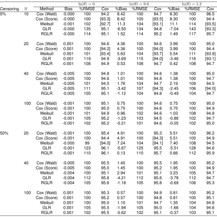
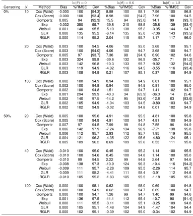
TABLE 3.1 : Empirical bias, percent ratio of MSE relative to Cox model and coverage probability for 95% C.I. forln(θ) = 0,0.6,1.2based on 5000 simulations and an underlying Weibull distribution for the survival times. . . 33 TABLE 3.2 : Empirical bias, percent ratio of MSE relative to Cox model and coverage

probability for 95% C.I. forln(θ) = 0,0.6,1.2based on 5000 simulations and an underlying Gompertz distribution for the survival times. . . 36 TABLE 3.3 : Empirical bias, percent ratio of MSE relative to Cox model and coverage

probability for 95% C.I. forln(θ) = 0,0.6,1.2based on 5000 simulations and an underlying Weibull distribution for the survival times with tied observations. 39

TABLE 4.1 : True log hazard ratio in each stratum and overall under the null and alterna-tive hypotheses. . . 51 TABLE 4.2 : Bias (% bias), percent ratio of MSE relative to one-step stratified Cox model

and coverage probability for 95% C.I. for overall log hazard ratioβ¯for 2 strata based on 5000 simulations. . . 53 TABLE 4.3 : Bias (% bias), percent ratio of MSE relative to one-step stratified Cox model

and coverage probability for 95% C.I. for overall log hazard ratioβ¯for 4 strata based on 5000 simulations. . . 54 TABLE 4.4 : Power comparisons among the competing methods based on 100 subjects

per treatment group and 50% censoring with 5000 simulations for 2 strata (top panel) and 4 strata (bottom panel). . . 55 TABLE 4.5 : Log hazard ratio estimates for the Colon cancer data example in Lin et al.

(2016). . . 55

TABLE A.1 : Trueθ values used in the simulation study under the alternative hypothesis for each combination of distribution, covariance structure,ρ¯, censoring and sample size per sequence (θ= 1under the null hypothesis.) . . . 61 TABLE A.2 : Power (%) for the hierarchical rank test (H-R), stratified Cox model with

base-line adjustment (SCB) and proposed multiple imputation with model aver-aging and ANCOVA (MIM A_{) under log-normal distribution based on 5000}

simulations. . . 61 TABLE A.3 : Power (%) for the hierarchical rank test (H-R), stratified Cox model with

base-line adjustment (SCB) and proposed multiple imputation with model aver-aging and ANCOVA (MIM A_{) under exponential distribution based on 5000}

TABLE A.4 : Power (%) for the hierarchical rank test (H-R), stratified Cox model with base-line adjustment (SCB) and proposed multiple imputation with model averag-ing and ANCOVA (MIM A_{) under gamma distribution based on 5000}

simula-tions. . . 62

LIST OF ILLUSTRATIONS

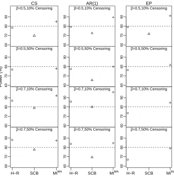
FIGURE 2.1 : Power comparison for the Hierarchical Rank test (H-R), stratified Cox model (SCB) and proposed multiple imputation with model averaging and AN-COVA (MIM A_{) under a log-normal distribution and varying assumptions}

for the true variance structure (compound symmetry (CS), first-order au-toregressive (AR(1)), equipredictability (EP), mean pairwise correlation of baseline and post-treatment values across the two periods (ρ¯ = 0.5,0.7) and percentage censoring (10%,50%), with 24 subjects per sequence. Stratified Cox model had non-convergence issues under CS structure with ¯

ρ= 0.5and 50% censoring, and under EP structure withρ¯= 0.5and 50% censoring, ρ¯ = 0.7 and 10% censoring and ρ¯ = 0.7 and 50% censoring, and hence power is not reported. . . 19 FIGURE 2.2 : Power comparison for the Hierarchical Rank test (H-R), stratified Cox model

(SCB) and proposed multiple imputation with model averaging and AN-COVA (MIM A_{) under an exponential distribution and varying assumptions}

for the true variance structure (compound symmetry (CS), first order au-toregressive (AR(1)), equipredictability (EP), mean pairwise correlation of baseline and post-treatment values across the two periods ( ¯ρ = 0.5,0.7) and percentage censoring (10%,50%), with 24 subjects per sequence. Stratified Cox model had non-convergence issues under EP structure with ¯

ρ= 0.7and 50% censoring, and hence power is not reported. . . 20 FIGURE 2.3 : Power comparison for the Hierarchical Rank test (H-R), stratified Cox model

(SCB) and proposed multiple imputation with model averaging and AN-COVA (MIM A_{) under a gamma distribution and varying assumptions for the}

true variance structure (compound symmetry (CS), first order autoregres-sive (AR(1)), equipredictability (EP), mean pairwise correlation of baseline and post-treatment values across the two periods (ρ¯ = 0.5,0.7) and per-centage censoring (10%,50%), with 24 subjects per sequence. . . 21 FIGURE 2.4 : Kaplan-Meier curves for the time to a symptomatic cardiac-related event

by treatment group from a 2×2 crossover trial; (a) is for period 1 and (b) is for period 2. . . 23

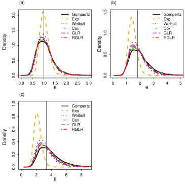
FIGURE 3.1 : Empirical densities of estimators from the Gompertz, exponential, and Weibull parametric survival models, Cox model, generalized log-rank (GLR) and refined GLR (RGLR) (5000 simulations for 20 subjects per group with 0% censoring and an underlying Gompertz distribution) with a true hazard ratio of (a) 1 (b) 1.82 (c) 3.32. A vertical line is drawn at the true hazard ratio. . 37 FIGURE 3.2 : Lung cancer data example: Kaplan-Meier curves for time to death

compar-ing test to standard chemotherapy by cell types. . . 40 FIGURE 3.3 : Lung cancer data example: Estimated hazard ratio and 95% confidence

interval comparing test to standard chemotherapy by cell types. . . 41 FIGURE 3.4 : Bladder cancer data example: Kaplan-Meier survival curves and estimated

hazard ratio and 95% confidence interval comparing placebo and chemother-apy by number of tumors removed at surgery. . . 43

FIGURE A.1 : Density curves for survival time under lognormal(µ = 0, σ = 1), whereµ andσdenotes the mean and standard deviation on the log scale, exponen-tial(rate=0.5) and gamma(shape=2, scale=0.7), respectively. . . 60

CHAPTER 1

I

Most statistical methods are developed based on large sample considerations. In real data

applica-tions, however, clinical trials and epidemiological studies with time-to-event outcomes do not always

meet the large sample size requirement due to various reasons. In fact, trials with small samples

are often encountered, due to reasons such as rarity of the disease and nature of the trial design

(e.g., an early phase or pilot clinical trial). Commonly used methods in a typical survival analysis

include Cox proportional hazards model (Cox, 1972) and parametric regression. Inference is

typi-cally based on large sample theory, and may not be appropriate under small samples. Crossover

trials also often have small samples, as every subject serves as his or her own control to help

achieve higher efficiency than parallel designs. However, there is a lack of existing methods for

an-alyzing crossover studies with time-to-event outcomes. We focus on three specific types of designs

with time-to-event response variables and small sample sizes: two-period two-treatment crossover

trials, two-group parallel designs in the setting of proportional hazards without stratification, and

two-group parallel designs with stratification and proportional hazards.

1.1. Background

1.1.1. Crossover Designs

Crossover designs compare treatment effects on the same subject over different treatment

peri-ods. For trials with limited recruitment, crossover designs are ideal to use for higher efficiency than

parallel designs. Under the commonly used two-period, two-treatment (2×2) crossover designs,

patients are randomized to one of two sequences, AB or BA, where A and B are the treatment

labels. A ‘washout’ period is included between the two periods to ensure no carry-over effects. The

use of a period-specific baseline measurement, which is taken before the subject is given the

treat-ment in each period, has been shown to increase statistical power (Chen, Meng, and Zhang, 2012;

Kenward and Roger, 2010; Senn, 2002). There are many existing methods for handling baseline

information in the analysis of crossover trials withcontinuous endpoints, including ignoring

base-line measurements, analyzing the change from basebase-line, using a function of the basebase-lines as a

2012; Hills and Armitage, 1979; Kenward and Roger, 2010; Metcalfe, 2010; Yan, 2013). Some

recommended methods for providing higher efficiency than others include analysis of covariance

(ANCOVA) and joint-modeling of the within-subject difference in treatment responses and

differ-ence in baseline responses (Mehrotra, 2014). The commonly used method, analysis of the change

from baseline, suffered from poor efficiency, as also discussed by Kenward and Roger (2010) and

Metcalfe (2010).

All methods mentioned above are for continuous endpoints, but crossover trials with time-to-event

endpoints are also commonly encountered in research. Existing literature for examining treatment

differences in crossover trials with censored time-to-event endpoints includes both

regression-based and test-regression-based approaches. France, Lewis, and Kay (1991) used stratified Cox regression,

where each subject was treated as a stratum. Feingold and Gillespie (1996) proposed an approach

based on the generalized Wilcoxon test. More recently, Brittain and Follmann (2011) proposed a

hierarchical rank (H-R) test, where each patient is assigned a rank based on whether and when he

or she has an event. The first ordering of the rank is determined by whether the individual has an

event during any of the two periods, and the second ordering of the rank is based on the times of

the events. A two-group Wilcoxon test is performed using the assigned ranks to test for the

treat-ment effect. Brittain and Follmann (2011) showed that the H-R test has similar or greater power

than both the Feingold and Gillespie’s method and stratified Cox method under certain censoring

patterns. However, none of these approaches utilizes baseline information, and whether and how

to utilize baseline information in crossover trials with time-to-event outcomes has not been studied.

1.1.2. Parallel Designs under Proportional Hazards without Stratification

In parallel designs with time-to-event outcomes comparing two treatment groups, the parameter of

interest is usually the hazard ratio, also referred to as relative risk. Under the proportional

haz-ards assumption, i.e., the hazard ratio is constant throughout time, it is conventional to use the

Cox proportional hazards model for estimation of relative risk and the log-rank test for hypothesis

testing (Cox, 1972). However, Cox regression is a large sample method, and may not provide an

appropriate result in small samples. Johnson et al. (1982) investigated the Cox model with one

binary indicator as the covariate, and found that in small samples, there are non-trivial differences

between the actual and asymptotic formula-based variances for the estimated log(hazard ratio).

bias when the true underlying survival distribution is misspecified. Therefore, it is important to

study analysis methods for failure time data in small samples, which are quite common in real data

applications. Early phase clinical trials usually have less than 100 subjects per treatment group

(Pocock, 1983), and cancer trials might have limited recruitment as well if the disease is rare.

Mehrotra and Roth (2001) proposed a method based on a generalized log-rank (GLR) statistic for

the 2-group comparison to improve estimation and inference of hazard ratio in small sample studies.

They showed that even though asymptotically the GLR method has similar performance to the Cox

approach, when the sample size is small, GLR is notably more efficient than the Cox approach,

in terms of mean squared error (MSE) for the log relative risk when there are no tied event times.

A deficiency in the GLR method is that it uses an unnecessary approximation involving nuisance

parameters which contributes to bias in the estimated hazard ratio. Furthermore, estimation of the

nuisance parameters follows a non-intuitive path. These collectively offer opportunities to improve

the GLR method in a tangible way with practical benefits.

1.1.3. Parallel Designs with Stratification and Proportional Hazards

In parallel designs comparing two treatments, when the risk of having an event is known to be

af-fected by a prognostic factor, such as gender or race, stratification is employed in the design stage.

Subjects are first divided into each stratum based on his or her prognostic factor characteristics,

and then within each stratum, randomized to receive one of the treatments. The goal is estimation

and inference involving the true‘overall’ hazard ratio, defined as the exponent of the weighted mean

of the stratum-specific true log hazard ratios using population relative frequency weights. Under the

assumption of proportional hazards in each stratum, stratified Cox model is used to analyze such

data. The stratified Cox model assumes that the hazard ratio is constant across strata, which is not

always true. If there exists a stratum-treatment interaction, the conventional stratified Cox model

tends to provide biased and less efficient results. Mehrotra, Su, and Li (2012) proposed a two-step

stratified Cox approach to allow for different hazard ratios across strata, and combine the

stratum-specific log hazard ratio by two weighting options, sample size weights and minimum risk weights

(Mehrotra and Railkar, 2000). The two-step analysis provides comparable power to the one-step

Cox analysis when there is no stratum-treatment interaction, but notably higher power when there

is an interaction. It also delivers a point estimator for the overall treatment effect with very small

hence not ideal for small studies.

1.2. Novel Developments

In this dissertation, we focus on developing methods for analyzing studies with time-to-event

out-comes in small samples, and specifically in three settings: 2×2 crossover designs with baseline

measurements, parallel designs for two group comparison under proportional hazards without

strat-ification, and stratified parallel designs under proportional hazards.

In Chapter 2, we propose a regression-based method using multiple imputation (MI) of censored

event times in conjunction with analysis of covariance (ANCOVA) to incorporate baseline

measure-ments into the analysis of crossover studies with time-to-event outcomes. In the imputation step,

we propose to fit multiple candidate survival models, and use frequentist model averaging to pool

the final results. Unlike Bayesian model averaging (Bates and Granger, 1969; Raftery, Madigan,

and Hoeting, 1997), which requires setting a prior probability to each candidate model, frequentist

model averaging does not need any priors (Buckland, Burnham, and Augustin, 1997; Burnham and

Anderson, 2003; Hjort and Claeskens, 2003). The final point estimator is obtained by averaging

across the imputations and a variance estimator is created that accounts for the uncertainty from

both model averaging and imputation. We show that there can be a great efficiency gain in

us-ing baseline information for time-to-event endpoints in crossover trials, compared to H-R test and

stratified Cox model. Furthermore, our proposed method delivers a point and confidence interval

estimate with small-to-no-bias of the treatment-ratio of geometric mean event times.. We

demon-strate the impressive performance of our proposed method through simulation studies and apply it

to data from a crossover trial studying a new drug’s effect on delaying a symptomatic cardiac-related

event during a 10-minute treadmill walking test.

In Chapter 3, we focus on the parallel design for the two group comparison without stratification

and propose a refined GLR (RGLR) method by replacing the‘approximate’ nuisance parameters

with‘exact’ counterparts in the original GLR statistic. We develop the RGLR statistic for settings

with and without tied event times, and show through extensive simulations that our proposed RGLR

method provides notably smaller bias than GLR, Cox and parametric models, and provides a high

relative efficiency and adequate 95% confidence interval coverage rate. We also provide further

the GLR statistic. Finally, we illustrate the method in two clinical trials studying lung cancer and

bladder cancer.

We further extend the RGLR method to allow for stratification factors in the analysis of a parallel

two-group design in Chapter 4. Instead of assuming a constant hazard ratio across all strata as done by

the commonly used stratified Cox model analysis, we allow the hazard ratio to vary across stratum,

and use two weighting schemes to combine the stratum-specific estimates of the log(hazard ratio).

We show through simulations that RGLR-based estimators provide smaller bias and higher relative

efficiency than both the conventional one-step and the two-step stratified Cox model estimator. We

apply the proposed method to a simulated data example for illustration.

CHAPTER 2

I

B

TIME

-

-

2.1. Introduction

Crossover designs are commonly seen in clinical trials to compare the treatment effects on the

same subject over different treatment periods. For trials with limited recruitment, crossover designs

are ideal to use for higher efficiency than parallel designs. The ability of each person to serve as

his or her own control also mitigates the influence of potential confounding factors. In commonly

used two-period, two-treatment (2×2) crossover designs, subjects are randomized to one of two

sequences, AB or BA, where A and B are the treatment labels. A ‘washout’ period is included

between the two periods to ensure no carry-over effects. The use of a period-specific baseline

measurement, which is taken before the subject is given the treatment in each period, is often

con-sidered. However, whether and how to use a baseline measurement is often challenging, given the

extra cost and the need to determine which statistical methods can be used to fully utilize the

in-formation from the baselines. For a 2×2 crossover trial, each subject has four responses: baseline

(i.e., pre-treatment) in period 1, post-treatment in period 1, baseline in period 2 and post-treatment

in period 2. There are many existing methods for handling baseline information in the analysis of

crossover trials withcontinuous endpoints, including ignoring baseline measurements, analyzing

the change from baseline, using a function of the baselines as a covariate, and joint-modeling of

baseline and post-treatment responses (Chen, Meng, and Zhang, 2012; Hills and Armitage, 1979;

Kenward and Roger, 2010; Metcalfe, 2010; Senn, 2002; Yan, 2013).

Mehrotra (2014) evaluated and compared 13 different methods for analyzing 2×2 crossover trials

to incorporate baseline measurements with continuous endpoints. Among all the competing

meth-ods, two methods were shown to have the highest efficiency: analysis of covariance (ANCOVA)

with the within-subject difference in baseline responses used as a covariate, and joint-modeling

of the within-subject difference in treatment responses and difference in baseline responses. The

commonly used method, analysis of the change from baseline, was shown to have poor efficiency,

All methods mentioned above are for continuous endpoints, but crossover trials with time-to-event

endpoints are also commonly encountered in research. For example, blood thinners like Warafin

are important in preventing outcomes such as blood clots and stroke, but can also induce

undesir-able increases in bleeding time from simple cuts or other injuries. In this setting, researchers are

sometimes interested in studying the effect of an experimental anticoagulant drug on bleeding time

using a crossover design with a baseline measurement at the beginning of each period. Kimchi et

al. (1983) and Markman et al. (2015) both studied a drug’s effect in a crossover trial with a

time-to-event outcome and collected baseline meausurements. However, neither incorporated the baseline

information into their analysis. Our motivating data example is a crossover trial studying a drug’s

effect in preventing cardiac-related symptoms in a treadmill walking test. The outcome of interest

for each subject is time to a specific cardiopulmonary event, with the outcome recorded as ’>10

minutes’ (i.e., right censored) if the event has not yet occurred after 10 minutes of observation.

Ex-isting literature for examining treatment differences in crossover trials with censored time-to-event

endpoints includes both regression-based and test-based approaches. France, Lewis, and Kay

(1991) used a stratified Cox regression, where each subject was treated as a stratum. Feingold

and Gillespie (1996) proposed an approach based on the generalized Wilcoxon test. More recently,

Brittain and Follmann (2011) proposed a hierarchical rank (H-R) test, which they showed to have

similar or greater power than both the Feingold and Gillespie’s method and stratified Cox method

under certain censoring patterns. The main idea behind the H-R test is that avoiding an event is

more clinically meaningful than delaying an event. Therefore, each patient is assigned a rank that

orders how much better an individual does on the novel treatment. The first order of ranking is

based on whether patients have an event, and second order of ranking is based on the times of

the events. Patients who do not have an event on either treatment receive the same rank. With

assigned ranks for everyone, a two-group Wilcoxon test is then performed to test for a treatment

effect. However, none of these Wilcoxon-type approaches utilizes baseline information.

In this research, we propose a regression-based method using multiple imputation (MI) of

cen-sored values and analysis of covariance (ANCOVA) to incorporate baseline measurements into

the analysis of 2×2 crossover studies with censored time-to-event response outcomes. There is

often uncertainty about the true underlying survival distribution in real data applications, and

mis-specification of the distribution can lead to a biased point estimator and/or inefficient analysis. To

fre-quentist model averaging to pool the final results from the ANCOVA step. Unlike Bayesian model

averaging (Bates and Granger, 1969; Raftery, Madigan, and Hoeting, 1997), which requires setting

a prior probability for each candidate model, frequentist model averaging does not require any

pri-ors (Buckland, Burnham, and Augustin, 1997; Burnham and Anderson, 2003; Hjort and Claeskens,

2003). To implement model averaging in the presence of multiple imputation, we need to account

for both the uncertainty from model averaging and imputation.

We show that there is a great efficiency gain in using baseline information for time-to-event

end-points in crossover trials compared to the H-R test and stratified Cox model. Furthermore, our

proposed method is also able to provide a point and confidence interval estimate of a meaningful

parameter of interest (treatment-ratio of geometric mean event times). Section 2.2 presents details

of the proposed method. In Section 2.3, we contrast the numerical performance of our proposed

method with that of the H-R test and stratified Cox model through simulation studies. Section 2.4

in-cludes results from applying the different methods to our motivating real data example. Section 2.5

includes conclusions.

2.2. Methods

We consider a 2×2 crossover trial with two treatments, denoted by A and B. Subjects are

random-ized to either the AB or BA sequence, with a wash-out period between period 1 and 2. LetXijk

andYijkdenote baseline and post-treatment event times, respectively, for subjectjfrom sequence

k in periodi, wherei = 1,2; j = 1,2, . . . , n; andk = 1,2. It is sufficient to assume that, after a

log transformation, (X1j1, Y1j1, X2j1, Y2j1)T and(X1j2, Y1j2, X2j2, Y2j2)T follow a multivariate

dis-tribution with different means and same variance-covariance structureΣ. We assume there is no

censoring at baseline, and in each period, subjects without a post-treatment event are censored at

the end of period, denoted by timeτ.

We propose a three-step procedure using multiple imputation and ANCOVA to estimate the ratio

of geometric means of the event times for treatment A relative to B, denoted as θ, and test the

null hypothesisH0 : θ = 1. For distributions that are symmetric on the log scale, the geometric

mean is equivalent to the median. Thus, our parameter of interest can be used to approximate the

ratio of median survival of the two treatments, which is commonly of interest in survival analysis.

details of which are given in the sub-sections below.

Step 1: Fit two candidate parametric event models, log-normal and Weibull, to impute the

post-treatment censored values sequentially, conditioning on the baseline event time in period 1 for

period 1 imputation, and both baseline event times and post-treatment event time in period 2 for

period 2 imputation.

Step 2: With the completed dataset from each candidate model, perform ANCOVA on the

log-transformed event times to estimatelogθand obtain its standard error.

Step 3: Average across thelogθestimates based on weights associated with Akaike information

criterion (AIC) from each parametric model fit to get a model averaged estimate and standard error,

and synthesize for overall point and confidence interval estimation across the multiply imputed

datasets using Rubin’s rule.

It is important to note that although we consider only two distributions in Step 1, our method can

be easily generalized to include more pre-specified candidate models in the imputation step. We

chose log-normal and Weibull because they are very flexible and in our experience provide

rea-sonable fitting models for capturing commonly seen event time data. Through numerical studies

in Section 2.3, we show that even averaging over a small number of models can deliver a good

performance.

2.2.1. Imputation

We generateM imputed data sets for each candidate model. LetZijk = 0,1denote treatment A

and B, respectively for subject j in periodi and sequencek. We impute the censored values in

period 1 first, and then impute the censored values in period 2. In them-th imputed data set, we

use the baseline value in period 1 and treatment indicator,Z1jk, as covariates and fit two candidate

parametric survival models, log-normal and Weibull, respectively, toY1jk.

logY1jk=βs,0+βs,1Z1jk+βs,2Us,1jk+σs,1Ws,1jk, (2.1)

where s = 1,2 denotes the log-normal and Weibull model, respectively, Ws,1jk is the error

dis-tribution and Us,1jk is the baseline covariate in thes-th model. W1,1jk has the standard normal

distribution for the log-normal distribution and W2,1jk has the standard extreme value distribution

the Weibull distribution; sample R code for implementation is provided in Appendix A. Equation (2.1)

is a representation of the log-normal and accelerated failure time (AFT) model framework for the

Weibull model that highlights the common linear regression model on the log-scale. For fitting the

parametric model, we analyze the log event times for the log-normal model and fit the traditional

Weibull model for the event times on the original scale. We use robust sandwich standard errors in

both candidate models to correct for potential model misspecification.

Letβˆ_s = ( ˆβs,0,βˆs,1,βˆs,2,σˆs,1)T andΣˆs denote the estimated coefficients and variance-covariance

matrix in thes-th candidate model, respectively. We drawβˆ∗_sfrom a multivariate normal distribution

N( ˆβs,Σˆs). For subject with a censored post-treatment value, we then impute a right-censored

value with an uncensored value by usingβˆs∗, treatment indicatorZ1jkand subject-specific period 1

baseline values in equation (2.1). The corresponding uncensored post-treatment values in period

1 are denoted byY_s,(m_1jk).

Now, with complete data in period 1, we can then use the observed/imputed post-treatment values

in period 1, baseline values in both period 1 and period 2 as covariates, to impute post-treatment

censored values in period 2 by fitting thes-th model,

logY2jk=αs,0+αs,1Z2jk+αs,2Us,1jk+αs,3Vs,2jk+αs,4R (m)

s,1jk+σs,2Ws,2jk, (2.2)

where U1,1jk = logX1jk, V1,2jk = logX2jk, R

(m)

s,1jk = logY

(m)

s,1jk for log-normal distribution, and

U1,1jk = X1jk, V2,2jk = X2jk, R

(m)

s,1jk = Y

(m)

s,1jk for Weibull distribution, and Z2jk is the treatment

indicator in period 2.

The imputation procedure described above for period 1 is now implemented using random draws

from the assumed multivariate normal distribution of the vector of estimated regression coefficients

in equation (2.2) for each of the two parametric models. The corresponding uncensored

post-treatment values in period 2 are denoted byY_s,(m_2jk).

2.2.2. ANCOVA

After each imputation, we have two sets of complete data on every subject from the two candidate

models, normal and Weibull. Each imputed dataset is analyzed using ANCOVA on the

times, ∆(_s,jkm) = logY_s,(m_1jk) −logY_s,(m_2jk) on the difference between baseline measurements, Djk =

logX1jk−logX2jkand the sequence indicatorQj.

∆(_s,jkm) =γs,0+γs,1Djk+γs,2Qj+s,jk, (2.3)

wheres,jk∼N(0, η2).

The point estimator from thes-th model in them-th imputed data set islog ˆθs(m) = ˆγ_s,(m₂)/2, which

is the logarithm of the ratio of geometric means for treatment A relative to B. The corresponding

variance estimate forlog ˆθ(sm)from thes-th model in them-th imputed data set isˆvs(m).

2.2.3. Model Averaging and Rubin’s Combination Rule

For overall estimation and inference, we first combine the two estimators from the candidate

mod-els in each imputed data set, then pool the model-averaged estimators from all the imputed data

sets and obtain the pooled variance estimate that accounts for both the uncertainty from model

averaging and imputation (Schomaker and Heumann, 2014).

For model averaging, we need to assign a standardized weight. There are many different options

for the choice of weights, including an information criterion (Buckland, Burnham, and Augustin,

1997), Mallows’ criterion (Hansen, 2007; Mallows, 1973) and cross-validation criterion (Hansen

and Racine, 2012). We propose to use the straightforward and commonly used Akaike Information

Criterion (AIC) (Akaike, 1974) to assign weights. LetIsdenote the AIC for the ANCOVA regression,

equation (3), from thes-th candidate model, then the weight is defined as (Buckland, Burnham, and

Augustin, 1997)

ws=

exp(−Is/2) P2

i=1exp(−Ii/2) .

The model averaged estimator in the m-th imputed data set is log ˆθ(m) ₌ P2

s=1wslog ˆθ (m)

s , and

the variance for the model averaging estimator is estimated by (Buckland, Burnham, and Augustin,

1997)

ˆ

Var(log ˆθ(m)) =

" ₂ X

s=1 ws

q

ˆ

Var(log ˆθ(sm)) + (log ˆθs(m)−log ˆθ(m))2 #2

. (2.4)

estimator calculated as (Schomaker and Heumann, 2014)

logθ¯ˆ= 1 M

M X

m=1

log ˆθ(m). (2.5)

When there is no model averaging, we can use Rubin (1987) to combine the results from multiple

imputation. As noted earlier, with the presence of model averaging, the uncertainty from both model

averaging and imputation needs to considered. The between-imputation variance is

vbtw = 1 M −1

M X

m=1

(log ˆθ(m)−logθ)¯ˆ2.

The within-imputation variance is the average of the estimated variance from equation (4) across

M imputed data sets

vwithin= 1 M M X m=1 ˆ

Var(log ˆθ(m)).

Therefore, the total variance of the estimator after multiple imputation is (Schomaker and Heumann,

2014)

vtotal=

M+ 1 M(M−1)

M X

m=1

(log ˆθ(m)−logθ)¯ˆ2+1 M M X m=1 " 2 X s=1 ws q ˆ

Var(log ˆθs(m)) + (log ˆθs(m)−log ˆθ(m))2 #2

.

(2.6)

To test the null hypothesisH0 : θ =θ0 (withθ0 = 1in our application), we carry out a t-test with

test statistic(logθ¯ˆ−logθ0)/

√

vtotal. To calculate the degrees of freedomd∗for the t-test, we follow

Barnard and Rubin (1999) so thatd∗= (1/d+ 1/dˆobs)−1, whered= (M−1)[1 +₍₁₊₁vwithin_/M)v

btw] 2_and

ˆ

dobs= (1−(1 + 1/M)vbtw/vtotal)(d_dcom+1

com+3)dcom, anddcomis the degrees of freedom for

¯ ˆ

θwhen there

are no missing values.

2.3. Simulation

2.3.1. Simulation Set-up

To compare the performance of our proposed approach to the H-R test and stratified Cox model,

we carried out a simulation study to examine type I error and power among all three methods.

times, in addition to the treatment indicator, as covariates in the stratified Cox model to make a

fair comparison. The H-R test, however, does not incorporate baseline information, and thus, we

used the method as is. We also examined the bias and 95% confidence interval (C.I.) coverage

probability from our proposed estimator; of note, the other two methods cannot deliver an estimate

of our parameter of interest (θ).

We simulated three underlying distributions for event times, namely log-normal, exponential and

gamma. Two of the distributions, log-normal and exponential (a special case of the Weibull),

are included in the candidate models in our method, while the gamma distribution is not. The

density curves for each of the three distributions are shown in Supplementary Figure A.1 in

Ap-pendix A. Under the log-normal distribution, for each of the N subjects in sequence AB and BA,

we generated correlated log event times from a multivariate normal distribution with mean

param-eter(0,logθ,0,0)T _{for AB sequence and (0,0,0,logθ)}T _{for BA sequence and common}

variance-covariance structure with common variance 1 and correlation coefficientsρ12, ρ13, ρ14, ρ23, ρ24, ρ34.

We considered three correlation structures, compound symmetry (CS), first-order autoregressive

(AR(1)), and equipredictability (EP), where ρ12 = ρ13 = ρ14 = ρ23 = ρ24 = ρ34 = ρ for CS,

ρ12=ρ23 =ρ34=ρ, ρ13 =ρ24=ρ2, ρ14 =ρ3for AR(1), andρ23=ρ14, ρ24=ρ13, ρ34 =ρ12for EP.

The correlation structures are as follows:

ΣCS =         

1 ρ ρ ρ

ρ 1 ρ ρ

ρ ρ 1 ρ

ρ ρ ρ 1

        

ΣAR=         

1 ρ ρ2 _ρ3

ρ 1 ρ ρ2

ρ2 _{ρ 1 ρ}

ρ3 _ρ2 _{ρ 1}

        

ΣEP =         

1 ρ12 ρ13 ρ14

ρ12 1 ρ14 ρ13

ρ13 ρ14 1 ρ12

ρ14 ρ13 ρ12 1

         .

We assumed no censoring in baseline event times in each period, and the post-treatment event

times were right-censored at timeτ. As discussed in the previous section, the parameter of interest

θis the ratio of the geometric means of the event times for treatment A and treatment B, and under

the log-normal distribution, it is equivalent to the ratio of median event times.

For the exponential distribution, we used copulas (Sklar, 1973) to generate correlated event times

from a multivariate exponential with mean(2,2θ,2,2)T for AB sequence and(2,2,2,2θ)T for BA

se-quence and common variance-covariance structure and correlation coefficients as specified above.

expo-nential distribution. Since copulas only preserves the rank correlation coefficient but not the linear

correlation coefficient (Genest and MacKay, 1986), the correlated exponential data follows

approx-imately, but not exactly, the specified variance-covariance structure.

To further illustrate the performance of our proposed method, we also considered an underlying

gamma distribution, which is not included in our two candidate models from the imputation step.

Specifically, we used a gamma distribution with scale of 0.7 and shape of 2 for subjects in

treat-ment B. Event times for subjects in treattreat-ment A was generated from a gamma distribution with

scale of 0.7θ and shape of 2. We again used copulas to generate the correlated event times.

For AB sequence, the simulated event times followed a multivariate gamma distribution with mean

(1.4,1.4θ,1.4,1.4)T, and for BA sequence, the event times follows a gamma distribution with mean

(1.4,1.4,1.4,1.4θ)T_{. Note that it can be shown that the ratio of arithmetic means is equivalent to the}

ratio of geometric means in the setting that event times in treatment A and B follow a gamma

distri-bution with the same shape parameter and ratio of scale parameter ofθ. Again, the event times in

the two sequences followed a common variance-covariance structure and correlation coefficients

as specified above.

We varied the sample size, percentage of censoring, θ, correlation structure, and compared the

performance of the different methods. Sample size per sequence was varied as N = 12,24,48,

and percentage of censoring was controlled by changing the time τ, to generate 10% and 50%

censoring for the total sample.

The mean pairwise correlation coefficientρ¯took values of 0.5 and 0.7. Under CS,ρ= ¯ρ. For AR(1),

ρ= 0.7forρ¯= 0.5 andρ= 0.83forρ¯= 0.7. For EP, we setρ12 = 0.6, ρ13 = 0.5, ρ12 = 0.4when

¯

ρ= 0.5, andρ12= 0.8, ρ13= 0.7, ρ12= 0.6whenρ¯= 0.7. We generatedM = 50imputed datasets

within each of the 5000 replications. Under the null hypothesis, θ = 1. Under the alternative

hypothesis, we chose a value ofθsuch that the power was about 80% for the H-R test, given the

true underlying distribution,Σ,ρ¯and percentage censoring.

2.3.2. Simulation Results

Table 2.1 reports type I error for the three distributions for the H-R test, stratified Cox model with

baseline adjustment and our proposed multiple imputation and model averaging and ANCOVA

under several scenarios when the sample size was 12 and 24 subjects per sequence with 50%

censoring, and had an inflated type I error when there were 24 subjects per sequence with 10%

censoring,ρ¯= 0.5and CS structure under exponential distribution. When the true distribution was

gamma, the stratified Cox model analysis was associated with inflated type I error under CS

struc-ture with 24 subjects per sequence andρ¯= 0.7, 10% censoring, and with 48 subjects per sequence

andρ¯= 0.7, 50% censoring. The H-R test and our proposed model averaging method controlled

type I error throughout all the scenarios considered. Table 2.1 also reports the bias in the estimate

of logθusing our proposed method under the null hypothesis. The bias was negligible under all

simulated scenarios.

Figures 2.1, 2.2 and 2.3 show the power for the three different methods forN = 24subjects per

sequence and different combinations of percentage censoring and variance-covariance structure

under the log-normal, exponential and gamma distributions, respectively; results for other sample

sizes are provided in Appendix A.

As shown in Figure 2.1, when the true distribution was log-normal, our proposed method always

provided a higher or similar power than the H-R test and stratified Cox model. For cases where the

H-R test or stratified Cox failed to deliver 80% power, our method was able to achieve power close

to or above 80%. The increase in power using our method was more significant under AR(1) and

EP structures than under CS structure. The power gain compared to the H-R test likely comes from

the fact that the H-R test fails to utilize baseline information. Likewise, our proposed method has a

substantially higher power than the stratified Cox model that adjusts for baseline covariates in part

because our method makes better use of the baseline information. In addition, the model averaging

aspect provides the flexibility of assuming more than one distribution and further improves the

efficiency of the analysis. Results from assuming only one distribution, either log-normal or Weibull,

is more prone to model misspecification in the imputation step.

Figure 2.2 displays the results when the true distribution was exponential. In this case, the true

variance-covariance structure and percentage censoring affected the relative performance of the

considered methods. When the true structure was CS, H-R test delivered higher power than the

other considered methods. Of note, CS structure usually does not capture the true correlation

pattern in most real data examples, since it assumes equal correlation among all pairs of

are a more realistic representation of the correlation structure in real data applications, our method

again showed a substantial power gain compared to the H-R test and stratified Cox model under

50% censoring. When the percentage censoring was 10%, our method delivered similar power

as the H-R test. For all the other scenarios, where the stratified Cox model did not have

non-convergence issues, our proposed method was consistently more powerful than the stratified Cox

model.

Finally, when the underlying distribution was gamma, our proposed method still provided higher

power than the stratified Cox model throughout all scenarios, but slightly lower power than the H-R

test under CS structures, as shown in Figure 2.3. Under AR and EP structures, using multiple

imputation, model averaging and ANCOVA approach delivered a more efficient analysis than both

the H-R test and stratified Cox model. Recall that the true distribution, gamma, is not included

as one of the candidate models in the imputation step; however, we are still able to provide a

comparably efficient result. Additionally, our proposed method is able to provide a point and CI

estimate of the treatment effect, while the other two methods do not.

Table 2.2 reports percentage bias and 95% C.I. coverage probability forlogθusing our proposed

method under the alternative hypothesis. Our method was able to control bias within 10% under

log-normal and exponential distribution. When the true distribution was gamma, it controlled bias

within 10% under 10% censoring, and under 50% censoring, bias was no larger than 11%.

Impor-tantly, the 95% C.I. coverage probability was maintained at or above the nominal level under all the

scenarios considered.

2.4. Data Application

We apply the three methods considered to a 2×2 crossover clinical trial of an investigation drug.

The trial recruited 40 subjects in total, and randomly assigned 20 to the placebo then drug sequence

and 20 to the drug then placebo sequence. The outcome variable was time until a symptomatic

cardiac-related event of interest during a 10-minute treadmill walking test. Each subject also had a

measurement at baseline before taking the treatment. Figure 2.4 displays the Kaplan-Meier curves

for post-treatment event times for placebo and drug in period 1 and period 2, separately.

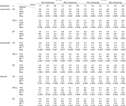
two-Table 2.1: Type I error (target=5%) for the hierarchical rank test (H-R), stratified Cox model with baseline adjustment (SCB) and proposed multiple imputation with model averaging and ANCOVA (MIM A_{) for log-normal, exponential and gamma distributions under the null hypothesisH}

0 :θ = 1 and bias in the estimate oflogθusing the proposed method (5000 simulations).

ρ= 0.5 ρ= 0.7

10% Censoring 50% Censoring 10% Censoring 50% Censoring

Distribution Σ XXXX XX

XXXX Method

N/seq

12 24 48 12 24 48 12 24 48 12 24 48

Log-normal CS H-R 4.6 4.3 4.9 4.4 4.3 4.8 4.5 5.0 4.3 4.6 4.8 4.8

SCB 4.5 4.4 4.9 NC 4.4 4.6 4.5 5.0 4.8 NC 4.5 4.9

MIM A _{4.3 4.8 4.9 2.4 3.9 4.9 4.8 4.9 4.8 1.9 3.8 4.2}

Bias -0.002 -0.002 0.000 0.001 0.002 -0.002 0.005 -0.002 -0.001 0.001 0.003 0.002

AR(1) H-R 5.0 4.0 4.8 5.0 4.7 4.8 4.7 4.8 5.0 4.8 4.6 4.8

SCB 4.2 4.4 4.5 NC 4.6 4.9 3.6 4.2 5.1 NC 4.6 4.7

MIM A _{4.6 4.4 4.7 2.8 3.8 4.8 4.7 4.7 5.0 2.6 4.0 4.5}

Bias 0.002 0.002 0.001 -0.007 0.000 -0.002 -0.001 -0.002 0.001 0.001 -0.002 -0.001

EP H-R 4.4 5.1 4.7 4.8 4.4 4.4 4.8 4.3 4.4 4.4 5.1 4.9

SCB NC 4.9 4.5 NC 4.7 4.6 NC 3.7 4.3 NC NC 4.8

MIM A _{4.5 5.0 5.0 2.7 4.4 4.7 4.7 4.4 4.7 1.4 3.2 3.7}

Bias -0.001 0.001 -0.002 0.001 0.001 0.001 0.001 -0.001 0.001 0.002 -0.000 0.002

Exponential CS H-R 4.8 4.8 5.0 4.9 4.5 4.8 4.7 4.6 5.0 4.1 4.3 4.3

SCB 5.1 (5.6) 4.6 NC 4.7 5.0 4.0 4.7 5.3 NC 4.4 5.0

MIM A _{4.7 5.0 4.4 2.2 3.8 5.1 4.4 4.8 4.5 1.8 2.9 4.0}

Bias -0.003 -0.002 0.001 -0.071 -0.006 0.002 0.001 -0.001 0.002 0.063 0.002 -0.002

AR(1) H-R 4.6 4.6 4.6 4.6 5.0 4.4 4.3 5.0 5.1 4.5 4.5 4.8

SCB NC 4.5 5.2 NC 4.7 4.6 NC 4.8 5.2 NC NC 4.7

MIM A _{4.9 4.7 4.2 2.0 3.5 4.2 4.4 4.5 4.5 1.9 2.9 3.0}

Bias -0.001 0.004 0.002 0.002 0.001 0.002 -0.001 -0.002 0.002 0.004 -0.001 -0.003

EP H-R 4.2 4.3 4.4 4.5 4.2 4.4 4.8 4.7 4.9 4.4 4.5 4.9

SCB NC 4.4 4.8 NC 4.3 4.5 NC NC 4.2 NC NC 4.2

MIM A _{4.4 4.3 4.5 1.8 3.3 4.3 4.4 4.6 4.6 1.4 2.1 2.4}

Bias -0.004 0.001 0.001 0.003 0.003 -0.001 0.002 -0.001 0.001 -0.015 0.001 0.001

Gamma CS H-R 4.2 4.4 4.7 4.4 4.4 4.6 4.2 4.7 4.4 4.1 4.8 5.1

SCB 4.2 4.9 4.6 NC 4.6 4.8 NC (5.9) 4.7 NC 4.9 (5.6)

MIM A _{4.5 4.7 4.9 4.2 4.7 5.0 4.7 5.0 4.8 3.2 4.4 4.8}

Bias 0.001 0.002 -0.002 0.001 -0.000 0.001 0.002 0.002 -0.000 -0.002 -0.003 0.002

AR(1) H-R 4.3 4.6 4.4 4.7 5.1 4.5 4.4 4.2 4.3 4.3 4.7 4.8

SCB 3.7 5.1 4.8 NC 4.1 4.5 NC 4.6 4.1 NC 4.1 5.1

MIM A _{4.7 5.1 4.6 3.8 4.6 4.7 4.9 4.7 4.1 3.3 4.6 4.6}

Bias -0.000 -0.000 -0.001 -0.006 0.001 0.000 -0.001 0.001 0.001 0.001 0.000 0.001

EP H-R 4.9 4.6 5.2 4.7 4.5 4.6 4.7 4.2 4.7 4.6 5.1 4.4

SCB 4.3 5.0 5.2 NC 4.4 4.5 NC 3.8 5.0 NC 3.7 4.8

MIM A _{4.7 4.3 4.9 3.5 4.7 5.0 4.8 4.7 4.5 3.0 3.9 4.0}

Bias 0.000 0.001 0.001 0.003 -0.000 -0.003 -0.000 -0.001 -0.001 0.001 -0.000 -0.001 Type I error more thanZ0.975standard errors above 5% level is in parentheses. NC: non convergence. CS: compound symmetry covariance structure. AR(1): first-order

autoregressive covariance structure. EP: equipredicability covariance structure.ρ¯: mean pairwise correlation.

tailed 5% level of significance to show a difference between the drug and placebo in delaying the

event of interest. On the other hand, stratified Cox model adjusting for period-specific baseline and

our proposed method deliver a p-value of 0.020, and 0.005, respectively. The ratio of geometric

mean of time to the cardiac-related event for patients taking the drug to patients on placebo was

estimated to be 1.67, with 95% C.I of (1.18, 2.35). The raw data from this trial are provided in

Table 2.3, and R code used to generate the analysis results for all the three methods are provided

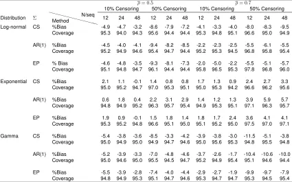
Table 2.2: Percentage bias and 95% C.I. coverage probability under the alternative hypothesis H1 :θ6= 1for the estimate oflogθusing the proposed method under log-normal, exponential and gamma distributions (5000 simulations).

ρ= 0.5 ρ= 0.7

10% Censoring 50% Censoring 10% Censoring 50% Censoring Distribution Σ XXXX

XX

XX_X

X Method

N/seq

12 24 48 12 24 48 12 24 48 12 24 48 Log-normal CS %Bias -4.9 -4.7 -3.2 -8.6 -7.9 -7.2 -4.1 -3.3 -4.0 -8.0 -8.3 -9.5

Coverage 95.3 94.0 94.3 95.6 94.4 94.4 95.3 94.8 95.1 96.6 95.0 94.9 AR(1) %Bias -4.5 -4.0 -4.1 -9.4 -8.2 -8.5 -2.2 -2.3 -2.5 -5.5 -6.1 -5.5 Coverage 95.2 94.9 94.6 95.4 94.7 94.4 95.2 95.3 94.5 96.8 95.8 95.4 EP % Bias -4.6 -4.8 -3.5 -9.3 -8.1 -7.3 -2.0 -5.0 -2.2 -5.5 -5.1 -5.7 Coverage 95.1 94.8 94.7 96.1 94.4 94.4 95.8 96.5 95.3 97.8 96.8 96.0 Exponential CS %Bias 2.1 1.1 -0.1 1.4 0.8 0.8 1.7 1.3 0.9 2.4 2.7 3.3

Coverage 95.0 95.2 94.7 97.0 95.3 95.1 95.0 95.3 94.2 96.6 96.2 95.6 AR(1) %Bias 0.6 1.8 0.4 2.2 3.1 2.9 1.4 1.2 1.3 3.9 5.9 5.7

Coverage 94.8 94.9 95.2 96.3 95.7 95.4 94.9 95.3 95.1 97.1 96.3 95.7 EP %Bias 1.9 0.9 -0.1 1.5 1.8 1.4 1.8 1.7 2.4 3.6 4.1 4.1

Coverage 95.3 95.2 94.8 96.6 95.1 95.0 95.1 95.2 95.0 97.5 97.0 97.1 Gamma CS %Bias -5.4 -3.8 -3.6 -8.5 -3.3 -4.2 -3.9 -3.8 -3.0 -11.5 -5.1 -3.8 Coverage 95.0 94.9 95.0 94.9 94.7 94.6 95.0 95.6 95.3 94.8 95.5 94.8 AR(1) %Bias -5.2 -3.9 -3.3 -7.0 -4.8 -4.6 -3.7 -2.6 -1.7 -10.4 -10.6 -10.0 Coverage 95.0 94.6 95.0 95.5 94.5 94.7 95.2 94.9 95.4 95.1 94.6 94.4 EP %Bias -5.5 -3.9 -2.8 -7.4 -4.0 -4.4 -2.9 -2.7 -1.9 -9.9 -9.7 -7.9 Coverage 94.8 94.9 95.3 95.1 94.7 94.6 95.3 94.7 94.7 95.3 94.5 95.4

CS: compound symmetry covariance structure. AR(1): first-order autoregressive covariance structure. EP: equipredicability covariance structure.¯ρ: mean pairwise correlation. True values ofθused for all the simulated scenarios are provided in Table A.1 in Appendix A.

2.5. Discussion

While there are many methods for analyzing crossover trials with continuous endpoints, there are

few studying crossover trials with time-to-event outcomes, which are often seen in practice. In this

paper, we have proposed a method using multiple imputation, assuming two candidate parametric

event time models, to impute censored post-treatment values. For each imputed dataset, ANCOVA,

with difference in period-specific baseline responses as a covariate, is applied to log-transformed

event times to estimate the log treatment-ratio of geometric means. Frequentist model averaging

with AIC weighting in conjunction with Rubin’s combination rule for multiple imputation is used for

overall estimation and inference. We showed that by utilizing baseline information, our method

pro-vided a more efficient or as efficient result than some other existing methods, including H-R test

and stratified Cox model, across different combinations of variance-covariance structures,

percent-age censoring and sample sizes. By using model averaging, we are able to provide a more flexible

mis-●

ρ=0.5,10% Censoring

60 70 80 90 CS ●

ρ=0.5,50% Censoring

60

70

80

90

●

ρ=0.7,10% Censoring

60 70 80 90 ● 60 70 80 90

H−R SCB MIMA

P

o

w

er (%)

ρ=0.7,50% Censoring

●

ρ=0.5,10% Censoring

60 70 80 90 AR(1) ●

ρ=0.5,50% Censoring

60

70

80

90

●

ρ=0.7,10% Censoring

60 70 80 90 ● 60 70 80 90

H−R SCB MIMA

ρ=0.7,50% Censoring

●

ρ=0.5,10% Censoring

60 70 80 90 EP ●

ρ=0.5,50% Censoring

60

70

80

90

●

ρ=0.7,10% Censoring

60 70 80 90 ● 60 70 80 90

ρ=0.7,50% Censoring

H−R SCB MIMA

Figure 2.1: Power comparison for the Hierarchical Rank test (H-R), stratified Cox model (SCB) and proposed multiple imputation with model averaging and ANCOVA (MIM A_{) under a log-normal}

dis-tribution and varying assumptions for the true variance structure (compound symmetry (CS), first-order autoregressive (AR(1)), equipredictability (EP), mean pairwise correlation of baseline and post-treatment values across the two periods (ρ¯= 0.5,0.7) and percentage censoring (10%,50%), with 24 subjects per sequence. Stratified Cox model had non-convergence issues under CS struc-ture withρ¯= 0.5 and 50% censoring, and under EP structure withρ¯= 0.5 and 50% censoring, ¯

ρ= 0.7and 10% censoring andρ¯= 0.7and 50% censoring, and hence power is not reported.

specification of the true underlying distribution. Furthermore, the H-R approach does not provide a

point estimator, while our regression-based method delivers an estimated ratio of geometric means

of event times for one treatment relative to the other with small or no bias and adequate 95% C.I.

coverage. The ratio of geometric means is a useful parameter in that it is equivalent to the ratio of

median event times under a log-normal distribution and other distributions that are symmetric on

●

ρ=0.5,10% Censoring

60 70 80 90 CS ●

ρ=0.5,50% Censoring

60

70

80

90

●

ρ=0.7,10% Censoring

60 70 80 90 ● 60 70 80 90

H−R SCB MIMA

P

o

w

er (%)

ρ=0.7,50% Censoring

●

ρ=0.5,10% Censoring

60 70 80 90 AR(1) ●

ρ=0.5,50% Censoring

60

70

80

90

●

ρ=0.7,10% Censoring

60 70 80 90 ● 60 70 80 90

H−R SCB MIMA

ρ=0.7,50% Censoring

●

ρ=0.5,10% Censoring

60 70 80 90 EP ●

ρ=0.5,50% Censoring

60

70

80

90

●

ρ=0.7,10% Censoring

60 70 80 90 ● 60 70 80 90

ρ=0.7,50% Censoring

H−R SCB MIMA

Figure 2.2: Power comparison for the Hierarchical Rank test (H-R), stratified Cox model (SCB) and proposed multiple imputation with model averaging and ANCOVA (MIM A_{) under an exponential}

dis-tribution and varying assumptions for the true variance structure (compound symmetry (CS), first order autoregressive (AR(1)), equipredictability (EP), mean pairwise correlation of baseline and post-treatment values across the two periods( ¯ρ= 0.5,0.7) and percentage censoring (10%,50%), with 24 subjects per sequence. Stratified Cox model had non-convergence issues under EP struc-ture withρ¯= 0.7and 50% censoring, and hence power is not reported.

For our model-averaging approach, we only used two candidate models, log-normal and Weibull, to

impute censored post-treatment values. More distributions can readily be used. The candidate

dis-tributions should include those that cover a spectrum of anticipated plausible shapes of the survival

distribution for the outcome of interest. The relative success of our method, like other applications

of multiple imputation, is not expected to perform well if the imputation model is grossly

●

ρ=0.5,10% Censoring

60 70 80 90 CS ●

ρ=0.5,50% Censoring

60

70

80

90

●

ρ=0.7,10% Censoring

60 70 80 90 ● 60 70 80 90

H−R SCB MIMA

P

o

w

er (%)

ρ=0.7,50% Censoring

●

ρ=0.5,10% Censoring

60 70 80 90 AR(1) ●

ρ=0.5,50% Censoring

60

70

80

90

●

ρ=0.7,10% Censoring

60 70 80 90 ● 60 70 80 90

H−R SCB MIMA

ρ=0.7,50% Censoring

●

ρ=0.5,10% Censoring

60 70 80 90 EP ●

ρ=0.5,50% Censoring

60

70

80

90

●

ρ=0.7,10% Censoring

60 70 80 90 ● 60 70 80 90

ρ=0.7,50% Censoring

H−R SCB MIMA

Figure 2.3: Power comparison for the Hierarchical Rank test (H-R), stratified Cox model (SCB) and proposed multiple imputation with model averaging and ANCOVA (MIM A_{) under a gamma}

distribution and varying assumptions for the true variance structure (compound symmetry (CS), first order autoregressive (AR(1)), equipredictability (EP), mean pairwise correlation of baseline and post-treatment values across the two periods (ρ¯= 0.5,0.7) and percentage censoring (10%,50%), with 24 subjects per sequence.

settings considered, and thus, more candidate models could potentially improve these results.

Al-though there is no upper limit on the number of models that can be fit, having an unnecessarily

large amount of models is also not recommended, as it may increase the overall computation time

without improving the power. It is also important to note that in order to properly use the model

av-erage approach to combine the parameter estimates, all of the candidate models need to estimate

Table 2.3: Event times (minutes) for a 10-minute treadmill test in a 2×2 crossover clinical trial.

Placebo-drug sequence Drug-placebo sequence Period 1 (placebo) Period 2 (drug) Period 1 (drug) Period 2 (placebo) Subject X1 Y1 X2 Y2 Subject X1 Y1 X2 Y2

1 1.5 1 1 1.5 2 1 1 1 2.5

3 6 4 3.5 >10 4 6 >10 2.5 2.5

5 1 1 1.5 4.5 6 3 2 1 0.5

7 3.5 1.5 0.5 3 8 2.5 2.5 1.5 2

9 0.5 1 3.5 8 10 2 2.5 2.5 3

11 6 10 6 >10 12 1.5 4.5 2.5 1

13 0.5 0.5 1 >10 14 3.5 5.5 4.5 9.5

15 1 1 1 2.5 16 1 2 2 >10

17 1.5 1 0.5 0.5 18 6 >10 5 3.5

19 1 1.5 2 4 20 2 3 1.5 1.5

21 5 5.5 3 1.5 22 1.5 2.5 1.5 0.5

23 2.5 5 6 4.5 24 1.5 3.5 2.5 3

25 5 5.5 4.5 6 26 3.5 9 6 6

27 1 2 2.5 8.5 28 2 5.5 3.5 8

29 5 5.5 3.5 2 30 2.5 2.5 1 0.5

31 0.5 1 2 7.5 32 2.5 3.5 2.5 4

33 5 4 2 2 34 5.5 3 1 0.5

35 0.5 0.5 1 1.5 36 3 5.5 5 0.5

37 1.5 2 3 3 38 0.5 1 1 5.5

39 6 4 1.5 0.5 40 2.5 5 2.5 0.5

Median 1.5 1.75 2 3.5 Median 2.5 3.25 2.5 2.5

X1: baseline response in period 1.Y1: post-treatment response in period 1.X2: baseline response in period

0 2 4 6 8 10

0.0

0.2

0.4

0.6

0.8

1.0

Time (a)

Drug Placebo

P

ercent of No Cardiac Ev

ent

0 2 4 6 8 10

0.0

0.2

0.4

0.6

0.8

1.0

Time (b)

Drug Placebo

P

ercent of No Cardiac Ev

ent