Theoretical Study of the 1 Self-Regulating Gene in
the Modified Wagner Model
Christophe Guyeux1,∗, Jean-François Couchot1, Arnaud Le Rouzic1, Jacques M. Bahi1and Luigi Marangio1
1 Université de Bourgogne Franche-Comté, Femto ST-Institute, UMR 6174 CNRS * Correspondence: [email protected]
Abstract:Predicting how a genetic change affects a given character is a major challenge in biology, and being able to tackle this problem relies on our ability to develop realistic models of gene networks. However, such models are rarely tractable mathematically. In this paper, we propose a mathematical analysis of the sigmoid variant of the Wagner gene-network model. By considering the simplest case, that is, one unique self-regulating gene, we show that numerical simulations are not the only tool available to study such models: theoretical studies can be done too, by mathematical analysis of discrete dynamical systems. It is first shown that the particular sigmoid function can be theoretically investigated. Secondly, we provide an illustration on how to apply such investigations in the case of the dynamical system representing the one self-regulating gene.
Keywords:Sigmoid functions; dynamical systems; gene networks
1. Introduction
Predicting the effect of a genetic change (differences in the DNA molecule) on a character of interest (which can be related to, e.g., human health, plant and animal production, or evolutionary
differences between species) remains a major challenge in biology [1]. This is mainly due to the fact
that cell physiology is heavily regulated by complex gene networks, which are able to compensate various genetic defects or environmental disturbances. Understanding how DNA variation translates to
observable (phenotypic) variation, due for instance to a modification of the conformation of proteins [2]
or DNA [3] a is of obvious importance, although very complex. Being able to tackle this complexity
relies, among other things, on our ability to develop realistic models of such gene networks.
There exist several kinds of biological interactions that can be modeled as gene networks (e.g., signal transduction, metabolism, or transcription regulation). The literature proposes several modeling
frameworks for each of them based on various biological hypotheses and different time scales [4–6].
An interesting subset of gene network models does not aim at predicting the behavior of a specific group of identified genes in an organism, but are rather used as a general abstraction of a gene network,
in order to study their evolutionary properties in individual-based simulations [7,8]. Although naive in
terms of biological hypotheses, these models are particularly important because they could contribute to unifying systems biology and evolutionary genetics.
The most popular framework in this field is the so-called “Wagner Model” (after [7,9]). This model
is an abstraction of the interactions between transcription factors (genes that regulate the expression of
other genes). The structure of then-gene network is encoded into an×nmatrix (Win the original
model, thereafter notedM), which is constant for an organism, and the status of the gene network
(the expression of thengenes of the network) is encoded into a vectorSof sizen. The dynamics
of the gene network over a finite number of discrete time steps is modeled as a system ofnlinear
difference equations, often written asSt+1=F(MSt), whereF(x) = [f(x1),f(x2), ...,f(xn)], in which
f is a scaling function. Then2elements of matrixMare real numbers representing the influence of
genejon genei(Mij <0 for repression,Mij >0 for up-regulation, and Mij =0 for the absence of
interaction). Self regulation is possible (and realistic),i.e.,Siican be different from 0. The purpose of
the scaling functionf is to ensure that gene expressionsSremain in their domain of definition. The
gene network starts from an initial vector of gene expressionsS0, generally set at an arbitrary level.
In the original setting from [9], gene expressions were discrete and could take only two values, -1
for no expression and 1 for an expressed gene, f(x)was thus a step function (f(x<0) =−1;f(0) =
0;f(x>0) =1). Alternative parameterization include e.g. scaling between 0 and 1 [10]. An overview
of the diversity of similar settings is provided in [11]. Recent implementations of the model consider
continuous gene expressions, and the step function was turned into a sigmoid, scaling gene expressions
between -1 and 1 (f(x) =2/(1+e−x)−1, [12], see [13] for a mathematical analysis). For more realism,
the sigmoid function can also be further modified to ensure that genes are only weakly expressed in
absence of regulators, by considering that f(0) =a<1/2, as in [14], and which is the model studied
below.
The main purpose of such models is to ensure that any combination M,S0 can be solved
computationally (e.g., as the state of the networkSTafterTtimesteps) within a predictable (most of the
time, constant) amount of time. This is of major importance in individual-based computer simulations
or other numerical studies in which the network structureMcan mutate and evolve over time. The
lack of mathematical tractability remains, however, problematic, as it makes it difficult to compare
simulation results with classical predictions from population and quantitative genetics models [15,16].
This is why, in this article, a mathematical analysis of the sigmoid variant of the Wagner gene-network model is presented, focusing on the simplest case, that is, one unique self-regulating gene. It is demonstrated that, in addition to classical numerical simulations, this model can be theoretically studied too, by the means of mathematical analysis of discrete dynamical systems. It is first shown that the particular sigmoid function, usually studied within this model, can be theoretically investigated, and such investigations are secondly partially applied to the dynamical system representing the one self-regulating gene. Finally, some ways to extend the analysis to the multiple gene case are sketched.
The remainder of this article is structured as follows. In the next section, the parameterized sigmoid function is deeply studied by the means of mathematical analysis. Effects of parameter changes on its shape are discussed too, and a systematic investigation of its fixed points is finally
provided. Section3, for its part, focuses on the discrete dynamical system of the modified Wagner
model. The one self-regulating gene model is next partially studied, in a particular situation and then in its most general formulation. This article ends by a conclusion section, in which the contribution is summarized and intended future work is outlined.
2. Studying the sigmoid function
We first provide some rationales about the sigmoid function usually considered in the variant
of the Wagner gene-network model studied here [14]. They will be used in the next section, when
studying the one self-regulating gene system.
2.1. Introducing the considered sigmoid
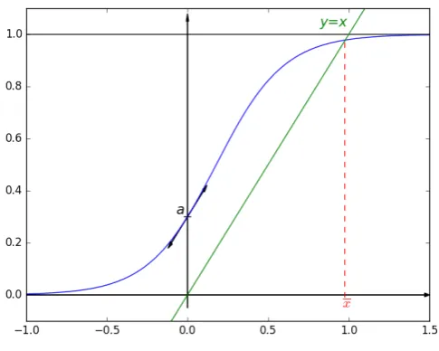
Let us considera∈]0, 1[and the particular sigmoid function defined by:
∀x ∈R,fa(x) = 1
1+λe−µx (1)
withλ= 1−a
a >0 andµ=
1 a(1−a) =
1 a+
1
1−a >1.
This function, and its parameters, have been chosen in order to have:
• a continuous increasing function,
• the limit of faasxapproaches negative infinity is 0,
• the limit of faasxapproaches infinity is 1,
• fa(0) =aand fa0(0) =1,
Figure 1.The chosen sigmoid function
fais a smooth function, with
∀x∈R,fa0(x) = λµe −µx
(1+λe−µx)2
>0. (2)
We can thus verify that fais strictly increasing. Additionally, we can reformulate this derivative,
to relate it to the logistic map:
fa0(x) =µfa(x) (1− fa(x)). (3) 2.2. Aboutλandµparameters
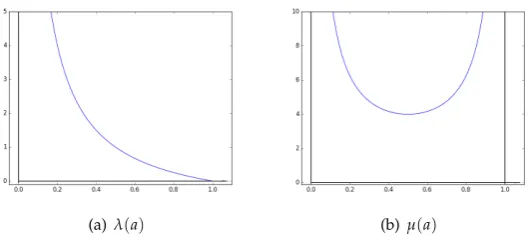
Let us now investigate the two parameters insidefathat both depend ona.λ(a) = 1
a−1 has a
curve depicted in Figure2(a).µ(a) = 1
a+ 1
1−a, for its part, has a derivative equal to:
µ0(a) = 2a−1
a2(1−a)2, (4)
whose variation table is as follows:
a
µ0(a)
Cµ
0 1
2 1
− 0 +
+∞ +∞
4 4
+∞ +∞
Let us thus remark thatλµ= 1
a2 >1, next that
λ
µ = (1−a)
2∈]0, 1[and finally thathis always
(a)λ(a) (b)µ(a)
Figure 2.Parameter dependence againsta
2.3. Fixed point of fa
One of the most important elements to study, when investigating the Wagner model, is the existence and meaning of fixed points. We will show that the fixed points of the one self-regulating
gene model are related to those of the modified sigmoid function fa, which are studied hereafter.
We can first remark that, as∀a∈[0, 1],fais continuous and such that fa([0, 1])⊂ fa([0, 1]), it is
thus a function mapping a compact convex set to itself. Due to Brouwer’s fixed-point theorem, fahas
at least one fixed point in[0, 1]. Let us prove that,
Theorem 1. ∀a∈[0, 1], fahas one unique fixed point inR, which is within[0, 1]. Proof. Let us first remark that, if fahas a fixed pointx, then it satisfies:
x= 1
1+λe−µx. (5)
Moreover, as fa(x) = xon the one hand, and fa(R) =]0, 1[on the other hand, we necessarily
have:
x∈]0, 1[. (6)
Additionally, 0<xandfais strictly increasing, so fa(0)< fa(x), which leads toa<x. To sum
up, iffahas a fixed pointx, then this latter satisfies:
0<a<x<1. (7)
Let us consider a fixed pointxforfa. So we have:
fa(x) =x⇐⇒ 1
1+λe−µx −x=0⇐⇒h(x) =
1
1+λe−µx 1−x−λxe
−µx =0.
Let us defineH(x) =1−x−λxe−µx, soxis a fixed point for faif and only if it is a zero ofH:H(x) =0.
Let us study the variations ofHfunction.
H0(x) =−1−λe−µx+λµxe−µx=λe−µx(µx−1)−1 H00(x) =−λµe−µx(µx−1)λµe−µx
=λµe−µx(2−µx) >0⇐⇒x< 2
µ
,
x
H00(x)
CH0
−∞ 2
µ +∞
+ 0 −
−∞ −∞
λe−2−1 λe−2−1
−1 −1
Depending on the sign ofλe−2−1,H0can be either negative on the wholeRset, or positive on a
bounded interval containing 2
µ. More precisely,
λe−2−1>0⇐⇒λ>e2⇐⇒1
a−1>e
2⇐⇒a
6 1
e2+1 ∈]0, 1[. (8)
• Ifa > 1
e2+1, thenH
0
6 0 onR, and we have lim
x→−∞H(x) =x→−lim∞1−x−λxe
−µx = +∞and
lim
x→+∞H(x) =−∞. So:
x
H0(x)
CH −∞ +∞ − +∞ +∞ −∞ −∞
Consequently, ifa> 1
e2+1, thenH(x) =0 has one unique solution,i.e.,fahas one unique fixed
point.
• Ifa6 1
e2+1, then there exist two real numbersx1andx2such that the following variation table
is satisfied forH:
x
H0(x)
CH
−∞ x1 2
µ x2 +∞
− 0 + + 0 −
+∞ +∞
H(x1) H(x1)
H(x2)
H(x2)
−∞ −∞ H 2 µ >0 – H 2 µ =
1−2
µ− 2λ
µe
−2
. Asµ>4, we deduce that 2
µ 6 1
2. Additionally,e
−2< 1
4 and
λ
µ = (1−a)
2∈]0, 1[, then2λ
µ e
−2< 1
2. As a conclusion,H
2 µ >0. AsH 2 µ
>0,His increasing on[2
µ,x2],Hdecreases on[x2,+∞[, and the limit ofHofx
asxapproaches+∞equals−∞, we can deduce thatH(x) =0 has an unique solution on
2 µ,∞
– We show thatH(x1)>0, and so fahas no fixed point on
−∞,2 µ
.
H0(x1) =0, thenλe−µx1(µx1−1)−1=0⇐⇒λe−µx1 = 1
µx1−1 . So:
H(x1) =−(λx1e−µx1 +x1−1)
=−
x1
µx1−1 +x1−1
= −(µx
2
1−µx1+1)
(µx1−1) .
Furthermore,H0
1 µ
=λe−1(1−1)−1<0, andH0is increasing on
−∞,2 µ
(asH00>0
on this interval). AsH0(x1) =0, we can deduce thatx1>
1
µ. Consequently,µx1−1>0. Let
j(x) =µx2−µx+1. Since 1+λe−µx1 >0, thusH(x1)is negative if and only ifj(x1)>0.
We now investigate the sign ofj.
As 0< 1
µ <x1< 2 µ 6
1
2, it is sufficient to studyjon the intervalI=
0,1
2
.
j0(x) =µ(2x−1), sojis strictly decreasing onI. The discriminant of the quadratic equation
j(x) =0 beingµ(µ−4)>0, the latter has two solutions µ±
p
µ(µ−4)
2µ , which are equal
whenµ= 4 (i.e. whena = 1
2). Note that only
µ−pµ(µ−4)
2µ may belong toI, and that
the latter is equal to1
2 − s 1 4− 1 µ= 1 2 − r 1
4−a(1−a)=
1
2 −
s
a−1 2
2
. We successively
have
1
2−
s
a−1 2 2 = 1 4 −
a−1 2 2 1 2+ s
a−1 2
2
= −a
2+a 1
2+
s
a−1 2
2
= −a(a−1)
1
2+
s
a−1 2
2
which is positive for eacha∈]0; 1[and less than 1
2. Thus
µ−pµ(µ−4)
2µ ∈]0; 1/2[and we
have:
x
j0(x)
j(x)
Cj
0 µ−
p
µ(µ−4) 2µ
1 2
− −
+ 0 −
1 1
1−µ
4
1−µ
4 0
Ifx1belongs to
"
0;µ−
p
µ(µ−4) 2µ
#
Figure 3.Evolution of the fixed-pointx(a)whenais varying
Let us show thatx1∈
"
µ−pµ(µ−4)
2µ ;
1 2
#
. Asa6 1
e2+1, we then havea−
1
2 <0, and so
s
a−1 2
2 = 1
2−a. Finally,
µ−pµ(µ−4)
2µ =a. As stated at the beginning of the proof,
sincex1is a root ofH,x1is a fixed point for faand thanks to (7).
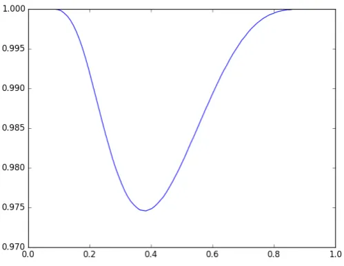
a<x1, and soj(x1)<0, asjis decreasing withj(a) =0. To put it in a nutshell,H(x1)>0.
A numerical simulation based on a dichotomic approach to solve the equation
x= 1
1+λ(a)e−µ(a)x
on[0, 1], leads to the curve depicted in Figure3.
Let us now establish the following result:
Proposition 1. For all x∈]0, 1[,|fa0(x)|<1.
Proof. As stated previously (equation (3)), fa0(x) =µfa(x) (1− fa(x)). So, we have
fa00(x) = µfa0(x) (1−fa(x))−µfa(x)fa0(x)
= µfa0(x) (1−2fa(x)).
Thanks to inequation (2) it can be deduced that fa00(x)shares then the same sign than 1−2faon
R, and consequently on[0, 1]where the fixed pointxis located. Furthermore,
1−2fa(x)60 ⇐⇒ fa(x)> 1
2 ⇐⇒
1
1+λe−µx >
1
2 ⇐⇒1+λe
−µx62
⇐⇒ e−µx6 1
λ ⇐⇒x> ln(λ)
Butln(λ)
µ >0⇐⇒λ>1⇐⇒ 1
a−1>1⇐⇒a6 1 2.
So, ifa> 1
2, then
ln(λ)
µ 60, and thus∀x ∈ [0, 1],x >
ln(λ)
µ . This implies that∀x ∈ [0, 1], 1−
2fa(x)60, and so∀x∈[0, 1],fa00(x)60. In other words, ifa>
1
2, then f
0
adecreases in[0, 1], and so:
∀x ∈[0, 1], 06 fa0(x)6 fa0(0) =a<1.
To sum up, ifa> 1
2, thenfais a contraction mapping such that|f
0
a|is bounded bya.
Let us now considera< 1
2, and ˇx=
ln(λ)
µ . ˇxis in[0, 1], as
ln(λ) µ =
ln
1−a
a
1 a(1−a)
6
1−a
a −1 1 a(1−a)
= (1−2a)(1−a),
and each term of the right-side product is in[0, 1]. Additionally, as 1−2fa(x)60⇐⇒x> ln(λ)
µ =xˇ
and as ˇx <1, we can deduce that the sigh of fa00, which is the one of 1−2fa(x), is negative forx>1.
Finally, limx−→+∞fa0(x) =limx−→+∞
λµe−µx
(1+λe−µx)2
=0. All these information are summarized below.
x
fa00
Cf0
a
fa0
Cfa
0 xˇ 1 +∞
+ 0 − −
1 1
µ 4 µ 4
0 0 fa0(1)
+ + +
aa
1 1 1/2
fa(1)
fa0(x)has a maximum in ˇx, but fa0(xˇ) =
µ
4 <1, sinceµ<4. In fact the functiona(1−a)has a
maximum ina=1/2. Since fa0is also positive on[0, 1]we have proven that|fa0(x)|<1, for allx∈]0, 1[.
From all the material detailed previously, we can thus conclude that,
Theorem 2. The unique fixed-point of fais an attractive one.
Proof. As|fa0(x)|<1, fais a contraction mapping. By applying the Banach fixed-point theorem, we can deduce again the existence and uniqueness, and in addition the exponential convergence of the dynamical system to this fixed point.
Note that:
1. The unique fixed-point can be found as follows: start with an arbitrary elementx0inRand define
2. Fora > 1/2, as|fa0(x)| < a, we can deduce that fa is Lipschitz continuous, with a Lipschitz
constant equal to a. As a well-known consequence, the convergence of the aforementioned
sequence is at least geometric, with a common ratio ofa. Fora<1/2 the same conclusion holds
but for a constantγ<1.
3. The 1-dimensional situation (n=1)
3.1. The discrete dynamical system under consideration
Let us firstly recall the general model to study gene networks. Letn ∈ N∗,M ∈ Mn(R)be a
square real matrix of sizen×n, and letX0∈Rn. We consider the discrete dynamical system:
(Σ) ∀k∈N,Xk+1=Fa(MXk) (9)
where
Fa: Rn −→ Rn
(x1, . . . ,xn) 7−→ (fa(x1), . . . ,fa(xn)).
Note that, most of the times,X0= (a, . . . ,a)T. We will now focus on its most simplest cases.
3.2. A fundamental case: M= (1)
Let us consider first thatn=1 and that the matrixMis the identity: M= (1). The(Σ)system
becomes:
(
x0 = a
xk+1 = fa(xk).
Let us recall that, if the recurrent sequenceuk+1= f(uk)converges, then the limit is a fixed point of f.
And, from the study of the previous section concerning the sigmoid fa, we know that this fixed-point
x(a):
1. exists and is unique,
2. is such that 06a<x(a)<1,
3. the convergence speed is geometric, of ratio equal toa(γ).
Asfais increasing, then the sequence(xk)k∈Nis monotonic. Being bounded, as faoutputs are in
]0, 1[, we can conclude that the sequence converges, and thus its limit isxa. Finally, ifx0<x(a), then
the sequence(xn)n∈Nincreases to its limit, and otherwise it decreases to its limitx(a), as depicted in
Figure4.
3.3. General 1-D case: M= (m)
In that case,(Σ)becomes:
(
x0 = a
xk+1 = fa(mxk), m∈ {0, 1}./
Let us introducega,m(x) = fa(mx).
3.3.1. Fixed points ofga,m
We first investigate the fixed points of ga,m, form > 0 : ga,m(x) = x ⇐⇒ x = 1
1+λe−µmx
⇐⇒ 1
1+λe−µmx(1−x−λxe
−µmx) =0. The casem<0 will be approach later in a different way.
As in the fundamental case of Section2.3, we are left to study the zeros of function Hm(x) =
1.0 0.5 0.0 0.5 1.0 1.5 0.0
0.2 0.4 0.6 0.8
1.0
y=x
x
a
(a)a=0.3,x0=0.1
1.0 0.5 0.0 0.5 1.0 1.5
0.0 0.2 0.4 0.6 0.8
1.0
y=x
x
a
(b)a=0.4,x0=1.5
Hm00(x) =λµme−µmx(2−µmx). H00m> 0 if and only if (1)m>0 and 2−µmx>0, or (2)m< 0 and
2−µmx<0. Both cases are equivalent tox < 2
µm. We then have the two following variations forH
0
m,
depending on the sign ofm. Ifm>0:
x
Hm00(x)
CH0
m
−∞ 2
µm +∞
+ 0 −
−∞
−∞
λe−2−1 λe−2−1
−1 −1
• Ifa> 1
e2+1, thenλe
−2−1 is negative and thenH0 60 over
R, and after the computation of
the limits ofHmasxapproaches±∞, we can deduce the following table of variations (which is
independent ofm):
x
Hm0 (x)
CHm
−∞ +∞
−
+∞ +∞
−∞
−∞
Consequently, ifa> 1
e2+1, thenHm(x) =0 has one unique solution,i.e.,ga,mhas one unique
fixed point.
• Ifa6 1
e2−1, then we obtain a curve similar to the fundamental case forHm.
x
Hm0 (x)
CHm
−∞ x1 2
µm x2 +∞
− 0 + + 0 −
+∞ +∞
Hm(x1) Hm(x1)
Hm(x2)
Hm(x2)
−∞ −∞ Hm
2 µm
>0
Let us show thatHm
2 µm
>0 for anym. It is successively equal to
Hm
2
µm
=
1− 2
µm− 2λ µme
−2
= µm−2 1+λe −2
µm
Whenm>0,Hm
2
µm
is positive if and only if
m> 2 1+λe
−2
We first note that
2 1+λe−2
µ =
a(a−1)2(a+e−2(1−a)
a =2(a−1)(a+e
−2(1−a))
Next, sincea6 1
e2−1, thena−1 is smaller than 0 and
2 1+λe−2
µ is smaller than 0 too. Since
mis positive, it is always greater than2 1+λe
−2
µ and thusHm
2 µm
>0.
So we can conclude thatga,mhas one single fixed point on
2 µm,+∞
.
As previously, we remark that H0(x1) =0= λe−µmx1(µmx1−1)−1, soλe−µmx1 = 1
µmx1−1 .
As a consequence,
Hm(x1) =−
x
1
µmx1−1 +x1−1
= −(µmx
2
1−µmx1+1)
(µmx1−1) .
Again as previously,H0m
1 mµ
=−1<0,Hm0 is increasing over
−∞, 2 µm
, andHm0 (x1) =0,
sox1> 1
µm. Consequently:
• ifm>0, thenµmx1−1>0, andHm(x1)has the opposite sign ofjm(x1) =µmx21−µmx1+1.
• elseµmx1<1, and soHm(x1)shares the same sign thanjm(x1).
Let us study the quadratic polynomialjm(x)onR. Its discriminant∆(jm)is equal toµ2m2−4µm=
µm(µm−4), and it has the following sign table:
m
∆(jm)
0 4
µ
+ 0 − 0 +
• Ifm∈
0,4
µ
, thenjm(x1) =µmx12−µmx1+1=µm
x1−1 2
2
−µm
4 +1. As 0<m<
4 µ, we
can conclude thatjm(x1)>0. SoHm(x1)<0, andHmthus changes twice its sign, respectively in
]−∞,x1[and in
x1, 2 µm
. Thusgm,ahas one fixed point in each of these two intervals.
• Ifm= 4
µ, then
h4
µ
(x1) = −(2x1−1)
2
(1+λe−4x1) (4x1−1),
which is of the size of 1−4x1. Butx1 > 1
mµ = 1
4 =⇒4x1>1=⇒1−4x1 <0. So, form=
• Ifm> 4
µ, then∆(jm)>0. Sojmis positive outside its two roots
1
2±
s
1
4 −
1
mµ. The largest one
is outsideI=
0;1
2
. Let us focus onz1= 1
2−
s
1
4−
1 mµ =
1 µm 1
2 +
s
1
4−
1 µm
. Since 06 1
µm 6 1 4
then 1
2 6
1
2 +
s
1
4−
1
µm61 and thus
1
µm6z16 2 µm.
– Ifµmis large (i.e., 1
µm is close to 0),z1is close to
1
µm. The left root of H,x1would be s.t.
x1≥z1andjm(x1)<0. In such a caseHm(x1)>0 and there is no fixed point.
– If µmis close to 4, z1is close to
2
µm. The left root of H, x1 would be s.t. x1 ≤ z1and
jm(x1)>0. In such a caseHm(x1)<0 and there is one fixed point in]−∞;x1[and one in
x1; 2 µm
.
– ifx1=z1,jm(x1) =0 and soHm(x1) =0. There is only one fixed pointx1ini−∞;µm2 i.
3.3.2. Casem<0
The existence of a unique fixed point can be proved without computations, however deeper investigation to establish the nature of this fixed pointed are necessary.
Lemma 1. ga,m(x)has at least one fixed point.
Proof. Suppose for an absurdum thatga,mhas no fixed points. Sincega,mis a continuous map and
ga,m(0) =awe have
Γ(ga,m):={(x,y):ga,m(x) =y} ⊂ {(x,y):x<y},
that is trivially false since there arex∈Rsuch thatx>ga,m(x), (for instancex =2/m).
Theorem 3. If m<0, then ga,mhas a unique fixed point.
Proof. LetP⊂R2be the subset of the fixed points ofga,m, i.e.P={(x,x)∈R2:ga,m(x) =x}; since
Pis a compact set, we can consider his minimump1∈P, that we may callthe first fixed point of ga,m. In
factP=Γ(ga,m)∩Γ(y=x)∩[0, 1]2, thusPis compact because is a finite intersection of close subsets
contained in a compact set ([0, 1]2).
Suppose for an absurdum to have another fixed pointp2; sincep1is the first fixed point, we have
p1< p2. Howeverga,mis a decreasing function on[0, 1], in fact
g0a,m(x) = λµme −µmx
(1+λe−µmx)2 ,
thus we have
p1=ga,m(p1)>ga,m(p2) =p2,
a contradiction that proves thatp1can be the only fixed point ofga,m.
As can be seen, the number of fixed-point ofga,m can be deduced theoretically, according to
the value of|g0a,m(x)|. Although technical, this latter can be done by using usual methods from the mathematical analysis.
4. Conclusion and future work
In this article, the objective was to show that gene-network models like the Wagner one, based on the iterations of some discrete dynamical systems defined using a sigmoid function, can be studied too theoretically. Iterations of the sigmoid function has been deeply studied in a first section, emphasizes the fact that the number of fixed points, their approximative location, and their attractivity, can be computed mathematically. Furthermore, we shown that each iteration of this sigmoid function tends to the fixed-point, no matter the initial condition. Elements showing how to extend this study to the complete one self-regulating gene has then be provided in a second section, showing the possibility of such studies. In future work, we intend to extend such investigations to a network of more than one gene. We will first deeply studied the case of 2-4 genes. Such investigations will then be extended to a larger number of genes, introducing qualitative methods that will depend on the shape of the considered matrix.
Conflicts of Interest:The authors declare no conflict of interest.
1. Bahi, J.M.; Guyeux, C.; Perasso, A. Chaos in DNA evolution. International Journal of Biomathematics (IJB)
2016,9(5), 1650076.
2. Guyeux, C.; Nicod, J.M.; Philippe, L.; Bahi, J.M. The study of unfoldable self-avoiding walks. Application to protein structure prediction software. JBCB, Journal of Bioinformatics and Computational Biology2015,
13(4), 1550009.
3. Pai, A.A.; Pritchard, J.K.; Gilad, Y. The genetic and mechanistic basis for variation in gene regulation. PLoS genetics2015,11, e1004857.
4. Bornholdt, S. Modeling genetic networks and their evolution: a complex dynamical systems perspective.
Biological chemistry2001,382, 1289–1299.
5. Barabási, A.L.; Oltvai, Z.N. Network biology: understanding the cell’s functional organization. Nature Reviews. Genetics2004,5, 101–113.
6. Polynikis, A.; Hogan, S.; di Bernardo, M. Comparing different ODE modelling approaches for gene regulatory networks.Journal of Theoretical Biology2009,261, 511–530.
7. Wagner, A. Does evolutionary plasticity evolve?Evolution1996,50, 1008–1023.
8. Fierst, J.L.; Phillips, P.C. Modeling the evolution of complex genetic systems: The gene network family tree.Journal of Experimental Zoology Part B: Molecular and Developmental Evolution2015,324, 1–12.
9. Wagner, A. Evolution of gene networks by gene duplications: a mathematical model and its implications on genome organization. Proceedings of the National Academy of Sciences1994,91, 4387–4391.
10. Masel, J. Genetic assimilation can occur in the absence of selection for the assimilating phenotype, suggesting a role for the canalization heuristic. Journal of Evolutionary Biology2004,17, 1106–1110. 11. Pinho, R.; Borenstein, E.; Feldman, M.W. Most networks in Wagner’s model are cycling. PloS one2012,
7, e34285.
12. Siegal, M.L.; Bergman, A. Waddington’s canalization revisited: developmental stability and evolution.
Proceedings of the National Academy of Sciences2002,99, 10528–10532.
13. Carneiro, M.O.; Taubes, C.H.; Hartl, D.L. Model transcriptional networks with continuously varying expression levels. BMC evolutionary biology2011,11, 363.
14. Rünneburger, E.; Le Rouzic, A. Why and how genetic canalization evolves in gene regulatory networks.
BMC Evolutionary Biology2016,16, 239.
15. Huerta-Sanchez, E.; Durrett, R. Wagner’s canalization model. Theoretical Population Biology 2007,
71, 121–130.