Tests and Problems of the Standard Model in
Cosmology
Mart´ın L´opez-Corredoira
Abstract The main foundations of the standardΛCDM model of cosmology are that: 1) The redshifts of the galaxies are due to the expansion of the Uni-verse plus peculiar motions; 2) The cosmic microwave background radiation and its anisotropies derive from the high energy primordial Universe when matter and radiation became decoupled; 3) The abundance pattern of the light elements is explained in terms of primordial nucleosynthesis; and 4) The formation and evolution of galaxies can be explained only in terms of gravi-tation within a inflation+dark matter+dark energy scenario. Numerous tests have been carried out on these ideas and, although the standard model works pretty well in fitting many observations, there are also many data that present apparent caveats to be understood with it. In this paper, I offer a review of these tests and problems, as well as some examples of alternative models.
Keywords Cosmology· Observational cosmology· Origin, formation, and abundances of the elements· dark matter· dark energy· superclusters and large-scale structure of the Universe
PACS 98.80.-k·98.80.E ·98.80.Ft·95.35.+d·95.36.+x·98.65.Dx Mathematics Subject Classification (2000) 85A40·85-03
1 Introduction
There is a dearth of discussion about possible wrong statements in the foun-dations of standard cosmology (the “Big Bang” hypothesis in the present-day version ofΛCDM, i.e. model which includes cold dark matter and theΛterm
Instituto de Astrof´ısica de Canarias, E-38205 La Laguna, Tenerife, Spain
Departamento de Astrof´ısica, Universidad de La Laguna, E-38206 La Laguna, Tenerife, Spain
in the energy, standing for dark energy or quintessence). Most cosmologists are pretty sure that they have the correct theory, and that they do not need to think about possible major errors in the basic notions of their standard theory. Most works in cosmology are dedicated to refining small details of the stan-dard model and do not worry about the foundations. There is still, however, a significant number of results in isolated and disconnected papers that are usually ignored by the leading cosmologists, and that are more challenging and critical of the standard model. My intention here is to bring together many of those heretical papers in order to help the more open-minded cosmologists to search the bibliography on tests and problems of the standard model.
In this paper, I will critically review the most important assumptions of the standard cosmological scenarios:
– The redshifts of the galaxies are due to the expansion of the Universe. – The cosmic microwave background radiation and its anisotropies come from
the high energy primordial Universe.
– The abundance pattern of the light elements is to be explained in terms of the primordial nucleosynthesis.
– The formation and evolution of galaxies can only be explained in terms of gravitation in the cold dark matter theory of an expanding Universe.
Some observations will be discussed or rediscussed in order to show that these facts were not strictly proven in some cases, but also, in other cases to show the solidity of the standard theory against certain tests.
There are many alternative theories. However, the purpose of this review is not to analyze the different theories, but to concentrate on the observational facts. In Ref. [1] I have reviewed theoretical ideas in cosmology that differ from the standard “Big Bang”. It would be interesting to extend this brief analysis to a wider literature survey, but that is a vast task well beyond the scope of the present review. Another review paper would be necessary to compile these alternative ideas and complete the present review. Here, I focus mainly in the compilation of facts and their interpretations.
Cosmologists do not usually work within the framework of alternative cos-mologies because they feel that these are not at present as competitive as the standard model. Certainly, they are not so developed, and they are not so developed because cosmologists do not work on them. It is a vicious circle. The fact that most cosmologists do not pay alternative theories any atten-tion and only dedicate their research time to the standard model is to a great extent due to the sociological phenomenon known as the “snowball effect” or “groupthink”[1]. This restricted view is unfair; therefore, I consider it ap-propriate to open the door here to further discussion of the results of the fundamental observations of cosmology.
I have chosen to review the general aspects of the foundations of cosmol-ogy as a whole instead of certain branches of it because I am interested in expressing the caveats and open questions as a whole in order to extract global conclusions on cosmology as a whole. It may also be that some of the caveats presented are no longer caveats, or that some of the observational measure-ments are not correct.Warning:I review only certain critical papers, and in a few cases I discuss them, but I take no responsibility for their contents.In most cases, I collect the information given by the different papers without any further research; I am conscious in any case that most of the most critical papers need further analysis in the problems they posit before reaching a firm conclusion on whether the standard model is correct or not. My own position is also neutral, I express no opinion on whether the standard cosmology is correct or not.
2 Redshift and expansion
2.1 Is a static model theoretically impossible?
A static model is usually rejected by most cosmologists. However, from a purely theoretical point of view, the representation of the Cosmos as Euclidean and static is not excluded. Both expanding and static space are possible for the description of the Universe.
Before Einstein and the rise of Riemannian and other non-Euclidean ge-ometries to the stage of physics, there were attempts to describe the known Universe in terms of Euclidean geometry, but with the problem of justifying a stable equilibrium. Within a relativistic context, Einstein[2] proposed a static model including a cosmological constant, his biggest blunder according to him-self. This model still has problems in guaranteeing stability, but it might be solved somehow. Narlikar & Arp[3] solve it within some variation of the Hoyle– Narlikar conformal theory of gravity, in which small perturbations of the flat Minkowski spacetime would lead to small oscillations about the line element rather than to a collapse. Boehmer et al.[4] analyze the stability of the Ein-stein static universe by considering homogeneous scalar perturbations in the context off(R) modified theories of gravity, and it is found that a stable Ein-stein cosmos with a positive cosmological constant is possible. Other authors solve the stability problem with the variation of fundamental constants [5, 6]. Another idea by Van Flandern[7] is that hypothetical gravitons responsible for the gravitational interaction have a finite cross-sectional area, so that they can only travel a finite distance, however great, before colliding with another graviton. So the range of the force of gravity would necessarily be limited in this way and collapse is avoided.
approach with a material tensor field in Minkowski space is given in Feyn-man’s gravitation[10], where the space is static but matter and fields can be expanding in a static space. Also worth mentioning is a model related to mod-ern relativistic and quantum field theories of basic fundamental interactions (strong, weak, electromagnetic): the relativistic field gravity theory and fractal matter distribution in static Minkowski space[11].
Olber’s paradox for an infinite Universe also needs subtle solutions, but extinction, absorption, and re-emission of light, fractal distribution of density, and the mechanism which itself produces the redshift of the galaxies might have something to do with its solution. These are old questions discussed in many classical books on cosmology (e.g., [12], ch. 3) and do not warrant further discussion here.
2.2 Does redshift mean expansion?
Lemaˆıtre[13] in 1927 and later Hubble[14] in 1929 established the redshift (z)– apparent magnitude relation of the galaxies, which gave an observational clue that the Universe is expanding. Hubble was cautious in suggesting this inter-pretation, but the following generations of cosmologists became pretty sure that the redshift of the galaxies following Hubble’s law is a definitive proof of expansion. This was due mainly to the absence of a good theory that explains the possible phenomenological fact of alternative proposals. General relativity provided an explanation for the cosmological expansion, while alternative pro-posals were not supported by any well-known orthodox theory. The expansion was preferred and the phenomenological approaches which were not supported by present-day theory would be doomed to be forgotten. This position would be right if our physics represented all the phenomena in the Universe, but from a deductive-empiricist point of view we should deduce theories from the observations, and not the opposite.
2.3 Alternative redshift theories
There are other mechanisms that produce redshift[15, 16] apart from space expansion or the Doppler effect. A bibliographical catalogue with hundreds of references before the ’80s to 17 classes of phenomenologies with untrivial redshifts is collected by Reboul[17](Sect. 1), the main idea being the “tired light” scenario.
different theories. There are several hypothetical theories which can produce this “tired light” effect. The idea of loss of energy of the photon in the inter-galactic medium was first suggested in 1929 by Zwicky[18] and was defended by him for a long time. Nernst in 1937 had developed a model which assumed that radiation was being absorbed by luminiferous ether. As late as the mid-twentieth century, Zwicky[19] maintained that the hypothesis of tired light was viable. But there are two problems[15]: 1) theφ-bath smears out the co-herence of the radiation from the source, and so all images of distant objects would look blurred if intergalactic space produced scattering, something that is incompatible with present-day observations[20]); 2) the scattering effect and the consequent loss of energy would be frequency dependent, which is again incompatible with what we observe in galaxies[21][22](S 4.1.1). Nonetheless, there are proposed solutions to these problems, as we will see in the following paragraphs.
Vigier[23] proposed a mechanism in which the vacuum behaves like a stochastic covariant superfluid aether whose excitations can interfere with the propagation of particles or light waves through it in a dissipative way. This avoids the two former difficulties of blurring and frequency dependence.
The photon-Raman interactions with atomic hydrogen[24, 25] also explains shifts that emulate the Doppler effect with light-matter interaction that does not blur the images. Or the redshift may be produced by a surface plasma that is undergoing rapid radial expansion giving rise to population inversion and laser action in some atomic species[26].
The justification of the shift in photon frequency in a low density plasma
could also come from quantum effects derived from standard quantum electrodynamics[27]. According to Paul Marmet and Grote Reber (a co-initiator of radio
astron-omy), quantum mechanics indicates that a photon gives up a tiny amount of energy as it collides with an electron, but its trajectory does not change[28](ap-pendix); this is called plasma redshift[29, 30, 31]. This mechanism also avoids blurring and scattering. In another model[32] the photon is viewed as an elec-tromagnetic wave whose electric field component causes oscillations in deep space free electrons, which then reradiate energy from the photon, causing a redshift. This new theoretical model is fundamentally different from Comp-ton scattering, and therefore avoids any problems associated with CompComp-ton scattering, such as image blurring. Potentially, this effect could explain the high redshifts of apparently nearby QSOs (Quasi Stellar Objects), since light travelling through the outer atmosphere of the QSO could be redshifted before leaving it. In order to explain galactic redshifts with long travel distances in the scattering, the density in the intergalactic medium should be 104 atoms/m3,
which is much higher than the density that is normally accepted (∼ 10−1
atoms/m3). However, the disagreement in the density of the intergalactic
medium is not necessarily a caveat in the hypothesis since our knowledge of the intergalactic medium is very poor, and there is also the possibility that intergalactic space is not so empty of baryonic matter.
that the shift in frequency of spectral lines is produced when light passes through a turbulent (or inhomogeneous) medium, owing to multiple scatter-ing effects. The new frequency of the line is proportional to the old one, the redshift does not depend on the incident frequency[34]. Redshift can also be explained in terms of non-linear optics, which assumes that the harmonic os-cillator model of light has to be extended somewhat by an extremely small anharmonic contribution[35].
The redshift might be due to a tired-light gravitational interaction of wave packets with curved spacetime[36, 37, 38]. The result is a redshift that is pro-portional to distance and to the square root of the density. Curvature pressure results from the non-geodesic motion of charged particles in the gravitational interaction.
Apart from the standard gravitational redshift derived from general rel-ativity [39, 40, 41, 16], with its own caveats, some theories are based on het-erodox ideas about gravitation. Broberg [42], for example, pointed out that a comparison between a quantizing scheme inherent in the Schwarzschild met-ric and observed redshifts from quasars shows that the contracted distances in the gravitational field are quantized in terms of the gravitational radii of the gravitating objects responsible for the field, whilst non-contracted dis-tances are not so quantized. Indeed, physicists have observed quantized states of matter under the influence of gravity: cold neutrons moving in a gravita-tional field do not move smoothly but jump from one height to another[43]. In Broberg’s view, this might be as important for modern quantum physics as the Michelson-Morley Experiment was for the introduction of special rela-tivity. Quantization therefore appears in systems with significant relativistic contraction (gravitational or Lorentz-contraction), such as de Broglie waves or, in the extreme case, photon energy packets at the speed of light. In generalized terms, this would mean that quantum physics has its origin in relativistically contracted fields, whereas the gravitational field can be scaled to particle di-mensions, with a constant surface energy density as the invariant parameter in the process. This might, for example, lead to the possibility of a topological transformation from the gravitational force to the strong nuclear force.
Amitabha Ghosh[44] proposed a phenomenological model of dynamic grav-itational interaction between two objects that depends not only on their masses and the distance between them, but also on the relative velocity and accelera-tion between the two. These velocity- and acceleraaccelera-tion-dependent interacaccelera-tions are termed “inertial induction”. The velocity-dependent force leads to a cosmic drag on all objects moving with respect to the mean rest-frame of a universe treated as infinite and quasi-static. This cosmic drag results in the cosmo-logical redshift of light coming from distant galaxies without any universal expansion. This force model leads to the exact equivalence of gravitational and inertial masses and explains many not well understood observed celestial and astronomical phenomena.
relativity + Mach’s principle + local conservation of energy. In SCC energy is conserved but energy-momentum is not. Particle masses increase with gravita-tional potential energy and, as a consequence, cosmological redshift, is caused by a secular, exponential increase of particle masses. The universe is static and eternal in its Jordan frame and linearly expanding in its Einstein frame. Fur-thermore, as the scalar field adapts the cosmological equations, they require the universe to have an overall density of only one third of the critical density and yet be spatially flat. Also in the theory a “time-slip” exists between atomic “clock” time on one hand and gravitational ephemeris and cosmological time on the other, which would result in observed cosmic acceleration.
There is more to be said about gravity and/or interaction with gravitons. In general relativity, dropping the restriction that a global time parameter exists, and assuming instead that the time scale depends on spatial distance, leads to static solutions, which exhibit no singularities, need no unobserved dark energy, and can explain the cosmological redshift without expansion[49]. Additional redshift can also be explained using Weyl geometry-gravitation[50, 51, 52, 53]. Interaction between gravitons and photons[7, 54, 55] might be re-sponsible for the redshift because it provides an energy loss mechanism that is not subject to the usual problem of making distant galaxy images fuzzy, and because it varies with (1 +z)−2which is closer to the observed rate of decrease
of surface brightness than any Big Bang model.
Instead of new ideas on gravitation, Roscoe’s [56] aim was to shed new light on classical electrodynamics. After abstracting from certain well-known symmetries of classical electrodynamics and showing that these symmetries are alone sufficient to recover the classical theory exactly and unadorned, he found that the classical electromagnetic field is then “irreducibly” associated with a massive vector field. This latter field can only be interpreted as a clas-sical representation of a massive photon. That is, it was demonstrated that existing classical theory is “already” compatible with the notion of a massive photon. He was then able to show that, given a certain natural assumption about how we should calculate the trajectories of this massive photon, the “quantized redshift phenomenology” can be understood in a simple and nat-ural way. Other new ideas rested not on new physics or new reinterpretations of old theories, but on effects predicted at present with standard physics. Also, Mosquera Cuesta et al. [57] propose a non-cosmological redshift that is non-linear in terms of the electrodynamical description of photon propaga-tion through weak background intergalactic magnetic fields. Indeed, Maxwell may have been the first to consider the possibility of non-conservative pho-ton behaviour. His original electromagnetic wave equation contained the en-ergy damping termσ0µ0(∂φ/∂t), where σ0 and µ0 represented the electrical
Furthermore, just to give further examples from the huge literature on the topic, there are explanations of non-cosmological/non-Doppler redshifts in terms of the local shrinkage of the quantum world[61]; or the time variation of the speed of light[62]; or proposals of a quantum long time energy redshift[63]: the energy is smaller owing to a quantum effect when the photon travels a very long time; chronometric cosmology[64, 65]; the variable mass hypothesis[66, 67, 3]; time acceleration[68], etc.
All these proposed mechanisms show us that it is quite possible to con-struct a cosmological scenario with non-expansion redshifts. Nonetheless, all these theories are at present just speculations without direct experimental or observational support.
2.4 Anomalous redshift in the laboratory and in the solar system
There are not many experiments that try to measure anomalous (neither Doppler nor gravitational) redshifts in the laboratory. One of these called my attention: Chen et al.[69] reported the observation of line shift increase with plasma electron densities: roughly ∆λ(nm)∼Ne(1018cm−3) for the HgI line
with λ= 435.83 nm. The dependence is also influenced by the temperature. This is justified by the authors by the difference in the atomic energy levels for higher electron density, leading to a longer wavelength. The Hg atomic levels embedded in a density environment are influenced by the free electron density. The electronic fields generated from free electrons compressed inside an atom screen the Coulomb potential of the atomic nucleus. The nuclear forces on the bound electrons are then diminished, while the repulsion of free to bound elec-trons is enhanced, so that the energy levels outside the nucleus are raised and the intervals of excited energy level 7s3S to 6p3P10 are diminished. Previous studies also pointed out this kind of redshifts[70]. My impression is that this emission redshift affects only to some lines and not the spectrum as a whole; in principle one would anticipate a dependence on wavelength. Moreover, it is not shown here that this can explain the absorption of a photon and its emission with redshift (like cosmological redshift), as Ashmore[30] thinks.
2.5 Observational tests for the expansion of the Universe
Nobody has ever directly observed a galaxy distance being increased with time. The motion of the putative expansion of the Universe is so slow that it is unmeasurable. The variation in the redshift of a galaxy is also very slow and difficult to measure. Sandage[75] proposed in 1962 to measure the expected
dz
dt = (1 +z)H0−H(z) (∼1 cm/s/yr), but it has not hitherto been possible
to meassure such a low acceleration. It would be possibly observable with a 40 m telescope over a period of ∼20 yr using 4000 h of observing time[76]. So, unfortunately, apart from the actual redshift of the galaxies, there are at present no direct proofs of the expansion. However, there are different indirect tests to verify whether the Universe is expanding or static:
1. Microwave background temperature as a function of redshift.
The Cosmic Microwave Background Radiation (CMBR) temperature can be detected indirectly at high redshift if suitable absorption lines can be found in high redshift objects. Hot Big Bang cosmology predicts that the temperature of the CMBR required to excite these lines is higher than at z= 0 by a factor (1 +z). For a static Universe, there is no specific CMBR model, but one may say that the temperature would be constant and equal to 2.73 K for all redshifts if there were a local CMBR origin, or possibly TCMBR(z) = 2.73(1 +z) K for a distant CMBR origin produced at a unique
distance and with a redshift due to tired light.
The CMBR temperature measured from the rotational excitation of some molecules as a function of redshift[77, 78] has been quite successful in prov-ing expansion: the results of Noterdaeme et al.[78] with the exact expected dependence onT =T0(1 +z) are impressive. However, there are other
re-sults that disagree with this dependence[79, 80]. The discrepancy might be due to a dependence on collisional excitation[77] or bias due to unresolved structure[80].
Nonetheless, there is another piece of evidence of the relationship T = T0(1 +z), which comes from the Sunyaev–Zel’dovich effect[81], the imprint
of galaxy clusters on the CMBR, and this does not have the problems noted in the previous paragraph. Therefore, if we accept these results, at least one can say with almost total confidence that a local origin of the CMBR in a static Universe is excluded, but the possibility of the origin of the CMBR at very high zwithin a static Universe is not excluded. 2. Time dilation test.
Clocks observed by us at high redshifts will appear to keep time at a rate (1 +z) times slower when there is expansion. By using sources of known constant intrinsic periodicity, we would expect their light curves to be stretched in the time axis by a factor (1 +z).
from selection effects. Other selection effects and the possible compatibility of the results with a wider range of cosmological models, including static ones, have also been pointed out[85, 86, 87, 88][37](Secc. 2)[89](Secc. 7.8). Moreover, neither gamma-ray bursts (GRBs)[90] nor QSOs[91] present time dilation, which is puzzling. However, with regard to this last fact, a variation in the quasar flux was found[92] in observations of more than 90 days with an average|dFV/dt|approximately proportional to (1 +z)−1,
although they used a sample of only 13 QSOs, without K-corrections. Fur-ther research is needed for the time dilation of quasars to arrive at firm conclusions.
3. Cosmic chronometers.
Measurements of the Hubble parameter ˙z using the variation of the age of elliptical galaxies with redshift as cosmic chronometers[93, 94] might be used to separate the different cosmological models. For the standard cos-mological model − z˙
1+z = H(z) = H0 p
Ωm(1 +z)3+ΩΛ, whereas for a
static model with tired light − z˙
1+z = H0, and for a static model with a
linear extrapolation of Hubble’s law with redshift − z˙ 1+z =
H0
1+z. The
dif-ferences in the predictions are huge, and the actual data[93, 94] favour the standard model and exclude a static universe. Regrettably, however, the assumptions made for cosmic chronometers are incorrect. It is not true that elliptical galaxies have a single stellar population, they have at least two distinct stellar populations, a young one and an old one, and the use of the Balmer break to measure the age of the galaxy reflects an age difference between both populations, not the maximum stellar age corresponding to the galaxy[95]. This is a serious problem for the use of cosmic chronome-ters as they are applied nowadays. Therefore, so long we have no accurate methods to determine the age of galaxies, this method is inapplicable. 4. Hubble diagram. It has been known for many decades that an
appar-ent magnitude (taking into account K-corrections) vs. redshift diagram for elliptical galaxies in clusters better fits a static than an expanding Universe[96]. This disagreement could, however, be solved by an increase of luminosity at higher redshift due to the evolution of galaxies.
For SNIa[97] or GRBs[98], for which it is supposed there is no evolution, the standard model works, provided that an ad hoc dark energy constant is included and we assume zero evolution and negligible extinction or selection effects (which are not universally accepted; [99, 100, 101]). Nonetheless, a static Universe may also fit those data[102, 103, 104, 105, 106]. By the way, there is anisotropy in the Hubble diagram (values ofH0andΩΛ) comparing
data of SNIa with z <0.2 from both Galactic hemispheres[107]. 5. The Tolman surface brightness test.
Hubble and Tolman[108] proposed the so-called Tolman test, based on the measurement of surface brightness. A galaxy at redshiftzvaries in surface brightness proportionally to (1 +z)−n, withn= 4 for expansion andn= 1
Lubin & Sandage[109], using the Tolman test up toz= 0.9, claimed in 2001 to have definitive proof of the expansion of the Universe. However, their claim, rather than being a Tolman test, was that the evolution of galaxies can explain the difference between the results of the Tolman test and their preferred model, which includes expansion. Lerner[110] observed that Lu-bin & Sandage used a very involved evolutionary k-correction scheme, with many adjustable assumptions and parameters to correct observed high-z surface brightness. These evolutionary and K-corrections are subject to uncertainty and cannot be used convincingly. Crawford[37] also pointed out that Lubin & Sandage performed an erroneous analysis to exclude the static solution, mixing Big Bang and tired-light models.
Furthermore, other more recent Tolman tests[110, 111, 112, 37], some of them up to redshifts of ∼ 5 and with different wavelength filters so that no K-corrections are necessary, favour a static Universe without the need for galaxy evolution, but they cannot exclude the standard scenario if evo-lution is allowed.
6. Angular size vs. redshift test.
The angular size (θ) of a galaxy with a given linear size[113] is very different according to whether we assume the standard model with expansion or a static Universe. Tests have been made by several authors[96, 114, 115, 104], and all of them, either in the radio, near infrared or visible, show, over a range of up to redshift 3, a dependence θ∼z−1, a static Euclidean effect
over all scales. This result cannot be reconciled with the standard cosmo-logical model unless we assume a strong evolution of galactic radii that just coincidentally happens to compensate for the difference[116]: galax-ies with the same luminosity should be six times smaller at z = 3.2 than at z = 0 [104]. It is usually further argued that elliptical and disc galax-ies have different evolutionary paths; that is right, but this difference was analysed and found to be compatible with a null one if we take into account the error bars of selection effects[104]. Angular-size test for massive disc-like galaxies also obtain a good fit for static universes without evolution according to some authors[89](Secc. 7.4)[117]. Neither the hypothesis that galaxies which formed earlier have much higher densities nor their luminos-ity evolution, merger ratio, or massive outflows due to a quasar feedback mechanism are enough to justify such a strong size evolution[104]; also, the velocity dispersion would be much higher than observed[104]. A static Universe is fitted without any ad hoc element. However, we must be cau-tious with this interpretation, because of the uncertainty in the galaxy size evolution.
There is yet another idea to be found in the literature about such a strong apparent evolution of galaxies: at high redshift, owing to the Tolman factor proportional to (1 +z)−4, the surface brightness of the galaxies is much
galaxies being observed at high redshifts), producing a downsizing illusion (dwarf galaxies apparently lift themselves above the sky at recent epochs). So far, there are no standard rods serving as physical objects without evo-lution. Double radio sources were proposed as standard rods[119] but there is also a strong inverse correlation between their absolute brightness and linear size, and some degree of evolution is not totally excluded[119, 120]. Ultra-compact radio sources were claimed in the past to be free of evolu-tionary effects, but they are now thought to show some signs of evolution as well[104, 121]. The huge size evolution necessary to fit an angular size test with an expanding universe is not understood[104] but still depends on our understanding of the galaxies rather than on pure cosmological ap-proaches. The ratio between gas mass fraction in clusters measured through X-ray and gas mass fraction (in the same clusters) measured through the Sunyaev–Zeldovich effect is proportional to the ratio of luminosity distance and angular distance, thus providing a method to derive indirectly the an-gular size (z), though this method assumes certain mass distributions in the cluster[122].
7. The galaxy number count magnitude test.
Differential galaxy number counts vs. galaxy K magnitude are fitted by the standard cosmological model[123], but also by the tired light Universe[89](Sect. 7.7). The same problem arises again: degeneracy between evolution and cosmological geometry.
8. UV surface brightness test.
Lerner[110] proposed a test of the evolution hypothesis that is also useful in the present case. There is a limit on the ultraviolet surface brightness (UV SB) of a galaxy because, when the surface density of hot bright stars and thus supernovae increases, large amounts of dust are produced to absorb all the UV except that from a thin layer. Further increase in the surface density of hot bright stars beyond a given point just produces more dust and a thinner surface layer, not an increase in UV SB. Based on this prin-ciple, there should be a maximum UV(at-rest) SB independent of redshift. This was analysed at high redshift[110, 104] and the result is that the in-trinsic UV SB magnitude of some galaxies would be prohibitively lower(i.e. much brighter) than 18.5 magAB/arcsec2 with the standard model. For a
static model, however, it would be within the normally expected range. Lerner[110] also argues why alternative explanations (lower production of dust at high redshift, winds, or other scenarios) are inconsistent. Nonethe-less, Lerner’s hypothesis of a maximum UV SB might be incorrect, so this should be further explored before reaching definitive conclusions about this test.
9. Alcock–Paczy´nski test.
Given a distribution of spherically symmetric objects with a radius along the line of sightsk=∆zd dcom(z)
dz and a radius perpendicular to the line of
sights⊥=∆θ(1+z)mdang(z) (m= 1 with expansion,m= 0 for static), the
ratioy≡ ∆z z∆θ
s⊥
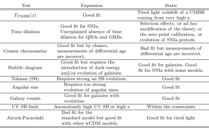
Table 1 Cosmological tests of the expansion.
Test Expansion Static
TCMBR(z) Good fit
Tired light redshift of a CMBR coming from very high z.
Time dilation
Good fit for SNIa.
Unexplained absence of time dilation for QSOs and GRBs.
Selection effects, or ad hoc modification of the theory or the zero point calibration,or evolution of SNIa periods.
Cosmic chronometer
Good fit but by chance,
measurements of differential age are incorrect.
Bad fit but measurements of differential age are incorrect.
Hubble diagram
Good fit but requires the introduction of dark energy and/or evolution of galaxies.
Good fit for galaxies.Good fit for SNIa with some models.
Tolman (SB) Requires strong an SB evolution. Good fit
Angular size Requires too strong
evolution of angular sizes. Good fit
Galaxy counts Good fit for galaxies with
evolution. Good fit
UV SB limit Anomalously high UV SB at high z Within the constraints
Alcock-Paczy´nski
Bad fit for the
standard model but good fit with other wCDM models.
Good fit for tired light
and the angular distance (dang(z)), and is independent of the evolution of
galaxies, but it also depends on the redshift distortions produced by the peculiar velocities of gravitational infall[124].
I have measuredy(z) by means of the analysis of the anisotropic correlation function of sources in several surveys[124], using a technique to disentangle the dynamic and geometric distortions, and also took other values avail-able from the literature. From six different cosmological models (concor-danceΛCDM, Einstein-de Sitter, open-Friedman Cosmology without dark energy, flat quasi-steady state cosmology, a static universe with a linear Hubble law, and a static universe with tired–light redshift), only two of them fitted the data of the Alcock & Paczy´nski’s test: concordanceΛCDM and static universe with tired-light redshift. The rest were excluded at a >95% confidence level. Analyses with further data using Baryonic Acous-tic Oscillations (BAO)[125] improve the test and give us a more accurate constraint: ΛCDM with standard values of parameters is excluded at 98% C.L., whereas static with tired light fits the data, but also an expanding Universe with zero-active mass or wCDM with ωdark energy =−0.60+0.30−0.27
andΩm= 0.45+0.21−0.19fits the data.
assume a very strong evolution of galaxy sizes to fit the data with the standard cosmology, whereas the Alcock–Paczynski test is independent of the evolution of galaxies but it does not show any preference for an expanding or static Universe yet.
2.6 Anomalous redshifts
Doubt might be cast upon the reality of the expansion as discussed above, but even in the case that it is definitively proven, this does not mean that all galaxies have a cosmological redshift, i.e. that all galaxies have a redshift due to the expansion. There might be some exceptions, which are known as “anomalous redshift” cases[15, 126, 127, 128, 129, 130, 131, 132, 133, 134]; that is, a redshift produced by a mechanism different from the expansion of the Uni-verse or the Doppler effect.
There are plenty of statistical analyses[128, 135, 136, 137, 138, 139, 140, 141, 142, 143, 144] showing an excess of high redshift sources near low redshift galax-ies, positive and very significant cross-correlations between surveys of galaxies and QSOs, an excess of pairs of QSOs with very different redshifts, etc.
There are plenty of individual cases of galaxies with an excess of QSOs with high redshifts near the centre of nearby galaxies, mostly AGN (Active Galactic Nuclei). In some cases, the QSOs are only a few arcseconds away from the centre of galaxies with different redshifts. Examples are NGC 613, 2237+0305, and 3C 343.1. In some cases there are even filaments/bridges/arms apparently connecting objects with different redshift: in NGC 4319+Mrk 205, QSO1327-206, NGC 3067+3C232 (in the radio). The probability of chance projections of background/foreground objects within a short distance of a galaxy or onto the filament is as low as 10−8, or even lower. The alignment of sources with
different redshifts also suggests that they may have a common origin, and that the direction of alignment is the direction of ejection. This happens with some configurations of QSOs around NGC 4235, NGC 5985, GC 0248+430, etc. Other proofs presented in favour of the QSO/galaxy association with different redshift is that no absorption lines have been found in QSOs corresponding to foreground galaxies (e.g. PKS 0454+036, PHL 1226), or distortions in the morphology of isolated galaxies.
The non-cosmological redshift hypothesis also affects galaxies differently from QSOs. Cases such as NGC 7603, AM 2004-295, AM 2052-221, etc., present statistical anomalies also suggesting that the redshift of some galaxies different from that of QSOs might have non-cosmological causes. Not all sup-porters of the non-cosmological redshift agree with this idea; for instance, Arp claimed that galaxies might have non-cosmological redshift because they de-rive from an evolution of ejected QSOs, while Geoffrey Burbidge only defended the non-cosmological redshifts in QSOs.
in the QSO research[145]. The standard paradigm model based on the existence of very massive black holes that are responsible for QSOS’ huge luminosities, resulting from to their cosmological redshifts, leaves many facts without ex-planation. There are several observations that lack a clear explanation; for instance[145], the absence of bright QSOs at low redshifts, a mysterious evo-lution not properly understood. There are alternative cosmological scenarios, such as the decelaration of time[146], that try to explain the problem without referring to an evolution effect in which the position of QSOs in the Hubble diagram is explained by an improper estimation of luminosity.
Calculations of the probabilities of the anomalous redshift cases being nor-mal background sources with cosmological redshifts and/or with amplifications due to gravitational lensing[134] indicate that some of the examples of appar-ent associations of QSOs and galaxies with differappar-ent redshifts may be just fortuitous cases in which background objects are close to the main galaxy al-though the statistical mean correlations remain to be explained, and some lone objects have a very low probability of being a projection of background objects. Nevertheless, these very low probabilities (down to 10−8or even lower,
assum-ing correct calculations) are not extremely low and, if the anomaly is real, one wonders why we do not find very clearly anomalous cases with probabilities as low as 10−20. Gravitational lensing seems not to be a general solution yet, although it explains some of the anomalies[147], and the requirement that the probabilities be calculated a posteriori is not in general an appropriate answer for avoiding or forgetting the problem.
3 Microwave Background Radiation
The CMBR has been interpreted as the relict radiation of an early stage of the Universe. Its black-body spectrum of 2.7 K reveals a very small dependence on sky position, of the order of∆T /T ∼10−5excluding the dipole due to the
motion of the Earth. Measurements of the anisotropies carried out by several teams of researchers over the last three decades have been claimed to provide information on the structural formation of the Universe, inflation in its early stages, quantum gravity, topological defects if any (strings, etc.), dark matter type and abundance, dark energy or quintessence, the geometry and dynamics of the Universe, the thermal history of the Universe at the recombination epoch, etc. Moreover, the CMBR has also become a source of accurate values for the parameters of this standard model of cosmology, which is usually called “precision Cosmology”[148]. The foundations of cosmology are thought to be definitively established, and now a quantitative science is pursued for which the fitting of the power spectrum of the distribution of CMBR anisotropies and a few other data, and which gives us the numerical values of the parameters in the equations governing the entire past, present, and future of our Universe.
3.1 Alternative explanations for the temperature of 2.7 K
There were predictions of CMBR temperature with origin different from the Big Bang [158] by Guillaume, Eddington, Regener, Nernst, McKellar, Herzberg, Finlay-Freundlich, and Max Born. Charles-Edouard Guillaume (Nobel laure-ate in Physics 1920) predicted in his article entitled “Les Rayons X” (“X-rays”, 1896) that the radiation of stars alone would maintain a background temper-ature of 6.1 K[159]. The expression “the tempertemper-ature of space” is the title of chapter 13 of “Internal constitution of the stars”[159, 160] by Eddington. He calculated the minimum temperature any body in space would cool to, given that it is immersed in the radiation of distant starlight. With no adjustable parameters, would be 3 K, essentially the same as the observed background (CMBR) temperature. Other early predictions[159], given by Regener[161] in 1933 or Nernst[162] in 1937, gave a temperature of 2.8 K for a black body which absorbed the energy of the cosmic rays arriving on earth. It was coun-tered that Eddington’s argument for the “temperature of space” applies at most to our Galaxy. But Eddington’s reasoning applies also to the temper-ature of intergalactic space, for which a minimum is set by the radiation of galaxy and QSO light. The original calculations half-a-century ago showed this limit probably fell in the range 1–6 K[163]. And that was before QSOs were discovered and before we knew the modern space density of galaxies. In this way, the existence of a microwave background in a tired light scenario[163, 164] was also deduced. But in a tired light model in a static universe the photons suffer a redshift that is proportional to the distance travelled, and in the ab-sence of absorption or emission the photon number density remains constant, we would not see a blackbody background. The universe cannot have an opti-cal depth large enough to preserve a thermal background spectrum in a tired light model[165] because we could not observe radio galaxies atz∼3 with the necessary optical depth. Therefore, it seems that this solution does not work, at least when the intergalactic medium instead of the shell of the galaxy is responsible for the tired light.
In the fifties, it was pointed out[166, 167] that if the observed abundance of He comes from hydrogen fusion in stars, there must have been a phase in the history of the Universe when the radiation density was much higher than the energy density of starlight today. If the average density of the visible matter in the Universe isρ∼3×10⁻³¹g/cm3and the observed He/H ratio by mass in it
is 0.244 (see§4), then the energy which must have been released in producing He is 4.39×10⁻¹³ erg/cm3. If this energy is thermalized, the black body
galaxy formation. The mechanism of thermalization in any of these cases is perhaps the hardest problem.
3.2 Alternative origin of CMBR
Dust emission differs substantially from that of a pure blackbody. Moreover, dust grains cannot be the source of the blackbody microwave radiation because there are not enough of them to be opaque, as needed to produce a blackbody spectrum. A solution for the blackbody emission shape might be unusual prop-erties of the dust particles: carbon needles, multiple explosions or big bangs, energy release of massive stars during the formation of galaxies, and so forth. The quasi-steady state model[170, 171] argues that there is a distribution of whiskers with size around 1 mm long and 10−6 cm in diameter with average ∼10−35g/cm3providing optical depthτ ∼7 up to redshift∼4. However, the presence of a huge dust density to make the Universe opaque is forbidden by the observed transparency up to z ∼4 or 5. A solution might be an infinite universe. An opaque Universe is required only in a finite space, an infinite universe can achieve thermodynamic equilibrium even if transparent out to very large distances. Somewhat similar to the proposal of whiskers is the pro-posal of the thermalization of “cosmoids”, cosmic meteoroids which are also observed in the solar system[172], or the proposal of emission by millimetre black holes[173].
Another possible explanation is the existence of an aether[174, 175], i.e. a material vacuum, whose emission gives the microwave background emission it-self. This aether would be an incompressible fluid according to Lorentz’s theory and its existence is in opposition to Einstein’s special relativity. Lorentz’s[176] invariant laws of mechanics in a flat space-time reproduce the standard ob-servational tests of general relativity provided that rest mass and light speed are not constant, so the final choice between Einstein’s and Lorentz’s theories cannot yet be regarded as settled according to Clube[174].
microwaves because farther radio sources with a given constant infrared emis-sion are fainter in the radio[179, 180]. However, there are some sources which are quite bright in radio at intermediate redshift: Cygnus A (z= 0.056) and Abell 2218 (z = 0.174). There is even a constant FIR/radio emission up to z = 1.5 [181, 182] and sources are observed at z = 4.4, so unless we have a problem of anomalous redshift in all these cases, which seems unlikely, Lerner’s ideas do not work.
Related to electrons, there are other discussions of alternative explanations of CMBR in the literature too. For instance, the radiation of electrons orbiting protons in atoms[183]. It is proposed that the atoms of hydrogen emit energy while in equilibrium owing to the orbiting of the electron around protons (which goes against the principles of quantum mechanics), thereby generating the background spectrum of 2.73 K. The atoms emit and absorb this radiation creating a background field with a blackbody shape.
Krishan[184] points out that, in addition to Thomson scattering, the ab-sorption due to the electron–electron, electron–ion and the electron–atom col-lisions in a partially ionized cosmic plasma would also contribute to the optical depth of the cosmic microwave background (CMB). The absorption depth de-pends on the plasma temperature and the frequency of the CMB radiation. The absorption effects are prominent at the low frequency part of the CMB spectrum. These effects, when included in the interpretation of the CMB spec-trum, may require a revised view of the ionization of the universe.
In “Curvature Cosmology”[185] the CMBR comes from the curvature-redshift process acting on the high-energy electrons and ions in the cosmic plasma. The energy loss which gives way to the spectrum of photons of the CMBR occurs when an electron that has been excited by the passage through curved spacetime interacts with a photon or charged particle and loses its excitation energy.
The origin must be very local in order to preserve the blackbody shape, or be non-redshifted, which seems problematic. Some proposals have even placed the origin of the CMBR within our own Galaxy, in the local bubble within 100 pc,[186], positing that the microwave background radiation stems in very large part in re-radiation of thermalized Galactic starlight. But the high level of isotropy, or the Sunyaev–Zel’dovich imprint of clusters of galaxies in the CMBR [187] or any possible correlation of the CMBR with galaxies would be puzzling in terms of such re-radiation.1
Navia et al.[188] find that there is an isotropic distribution of cosmic rays with energy>6×10¹⁹eV, so they should come from distances greater than 50
Mpc, and the cosmological interpretation of the CMBR does not allow these cosmic rays to travel distances ≥ 50 Mpc [189, 190]. However, Abraham et al.[191] claim that an isotropic distribution of these cosmic rays is rejected with>99% C.L. and that the most probable sources are nearby AGN. Kashti & Waxman[192] also claim that the distribution of these high energy cosmic
1 This has indeed not been found yet, since the measurements of the cross-correlation of
rays is inconsistent with isotropy at∼98% CL, and consistent with a source distribution that traces LSS, with some preference to a source distribution that is biased with respect to the galaxy distribution.
In my opinion, at present there is no satisfactory alternative scenario that does not have a problem in explaining the microwave background radiation, so the standard scenario seems to be the best solution, although also with some discussions about its plausibility in some skeptical literature.2 Nonetheless,
one’s mind should not be definitively closed against other options. The hot primordial Big Bang is only a hypothesis that should not be definitively con-sidered as a solid theory just because of the Microwave Background Radiation.
3.3 Microwave Background Radiation anisotropies
Another fact is the existence of certain anisotropies in CMBR. There are still some authors who doubt this fact, pointing out that there are spurious tem-perature anisotropies that are comparable with the entire signal[195, 196, 197], or testing the null hypothesis that the Time-Ordered-Data (TOD) were con-sistent with no anisotropies when hourly calibration parameters were allowed to vary, i.e. that sky maps with no anisotropies outside the galactic band other than the dipole were a better fit to the uncalibrated TOD than those from the official analysis [198]. In my opinion, these analyses cannot be correct. The fact that the same anisotropies have been found by many different experiments and by different teams leaves no doubt in my mind that the anisotropies are real.
The first predictions of CMBR anisotropies were wrong. One predicted ∆T /T to be one part in hundred or thousand [199]; however, this value could not fit the observations, which gave values hundreds of times smaller, so non-baryonic dark matter was introducedad hocto solve the question.
CMBR analyses in the last two decades have concentrated on anisotropies on small angular scales, smaller than the angular resolution of several degrees achieved by COBE-DMR in the ’90s. The power spectrum of the anisotropies of the experiments BOOMERANG and MAXIMA-1 showed a first peak at the Legendre multipole ` ≈200,[200, 201] corresponding to angular scales of ≈1.2◦, which was interpreted as a discovery of the previously predicted
acous-tic peaks in a flat Universe withΩ=Ωm+ΩΛ= 1, the greatest contribution
coming from a dark energy component ofΩΛ = 0.7 (see review in Ref. [202]
and references therein for further comments). Indeed, there are two parts in the comparison of theoretical predictions and observations: a successful one, and a half-successful/half-failed one. The totally successful prediction was the qualitative shape of the power spectrum containing several peaks: For instance,
2 For instance, the number of (CMBR) photons is much (109 times) higher than the
Peebles & Yu[203] had predicted a CMBR power spectrum with fluctuations, the acoustic peaks, from the hypothesis of primaeval adiabatic perturbations in an expanding universe. However, the position of the first peak was not at the expected position when first measured: already in the mid-’90s the posi-tion of the first peak was determined to be ` ≈200 with other experiments to measure small angular resolution anisotropies before BOOMERANG or MAXIMA-1 but with smaller sky coverage (Ref. [204] and references therein). De Bernardis et al.[200] and Hanany et al.[201] just added a refinement in the measurement of the position of the first peak but they were not its discoverers. White et al. in 1996 [204] realized that the preferred standard model of the time (an open Universe withΩ=Ωm≈0.2 and without dark energy) did not
fit the observations, so that they needed a largerΩ. This was one of the ele-ments, together with SNIa observations, and the age problem of the Universe, that would encourage cosmologists to include the new ad hoc element: dark energy. Between 1997 and 2000 this change of mentality in standard cosmology was produced, and then, in 2000, with the results of the new BOOMERANG and MAXIMA-1 experiments, cosmologists were proud to announce that new observations were giving exactly the results they expected. In any case, just paying attention to the first analyzes of the first peak in the mid-’90s, I would attribute a half-success to the prediction because, even though they failed to fit the observations with the preferred standard model of a curved open Universe at that time, the idea of a flat Universe was also presented as a possibility in the ’90s, and indeed a possibility preferred by inflationary paradigms. The po-sition of the other peaks would also serve to constrain the cosmological models. The acoustic peaks on angular scales of 1 deg and 0.3 deg were predicted with the second peak nearly as high as the first one in `(`+ 1)C`/(2π) [205, 206].
Later, as data became available, its amplitude was reduced and the positions of the other peaks and their relative heights were also constrained from the model with a higher agreement with the data (e.g. Ref. [207]).
More recently, the analysis of CMBR polarization anisotropies (e.g. Ref. [209]) has also provided strong support for the standard cosmology. This in-dicates the way in which the CMBR is polarized owing to the scattering of free electrons. Photon diffusion into regions of different temperatures are pos-sible only when the plasma becomes sufficiently optically thin; these diffused photons could then scatter only while there are still free electrons left. Since photons could not diffuse too far, polarization cannot vary much over very large angular scales.
Given this history of CMBR analyses, it is difficult to accept that our ob-servations reproduce “predictions”. Nonetheless, whichever comes first, theory or observation, the fact remains that we have now a cosmological model that is able to fit the CMBR power spectrum C` quite accurately. It is usually
thought that this may not happen by chance, given the apparent complexity of the power spectrum shape, whereas the six3parameter cosmological model
3 Plus many other parameters which introduce second-order changes. And, even so, there
is a degeneracy in the solutions with different values ofH0and ΩΛ: CMBR data, and the
exis-is relatively simple[209, 210], but thexis-is exis-is not correct, as I will explain in the following paragraphs.
Some critics of the standard model[211] claim that there is little value in the fact that the standard cosmological model might fit some observational cosmological data if the number of free parameters in the model were compara-ble to the number of independent parameters characterizing the observations. For instance, Ptolemaic geocentric astronomy may fit the observations of the orbits of the planets but with too high a number of free parameters in the theory. The principle of Occam’s razor tells us that a theory is better when the number of free parameters is low. Occam’s razor can indeed be under-stood with a Bayesian analysis, in which it is tested how probable a model is with a given number of free parameters with respect to other models with a higher number of free parameters[212, 213]. Otherwise, if a theory has a high number of free parameters, it loses credibility because it is always possible to create a “false” model to fit some data when the number of free parameters is comparable to the number of degrees of freedom in the data. Philosophers of science, when talking about cosmology, associate this approach with “instru-mentalism” (e.g., Ref. [214]). And saying that the power spectrum contains hundreds of independent parameters for a given resolution is not correct, be-cause the different values of C` for each ` are not independent in the same
sense that hundreds of observations of the position and velocity of a planet do not indicate hundreds of independent parameters. Indeed, the information on the orbit of planet is reduced to only six Keplerian parameters.
For the reasons just given, understanding how much information is in the power spectrum is important for key questions in the discussion of the fun-damentals of cosmology. There are indeed two main points which should be clarified:
1. Are the oscillations something atypical in a power spectrum? That is, should we consider the fact the power spectrum contains oscillations a successful prediction of the standard cosmological model that cannot be produced by any other means?
2. How much information is contained in the power spectrum? That is, how many free parameters in a function are necessary to fit the CMBR power spectrum? Should we consider the fitting of the power spectrum with a model of six free parameters as a validation of the standard cosmological model?
For the answer to the first question, we must bear in mind that the presence of peaks in the power spectrum is a rather normal characteristic expected from any fluid with clouds of overdensities that emit/absorb radiation or interact
gravitationally with the photons, and with a finite range of sizes and distances for those clouds. Apart from the standard cosmological model, other scenarios may also follow these conditions. The interpretation of “acoustic” peaks is just a particular case; peaks in the power spectrum may be generated in scenarios that have nothing to do with oscillations due to gravitational compression[215, 216].
For the second question, we must note that a simple polynomial function with no physical interpretation with six free parameters is able more or less to reproduce the two-point correlation function (the Fourier transform of the power spectrum), giving very good fit for at least the first two peaks of the power spectrum[216]. The fact the standard model is able to fit the CMBR anisotropies with a model with six free parameters is astonishing but it would be much more surprising if it could fit it without free parameters or with only one or two free parameters fitted to the power spectrum. Certainly, the same parameters which are used to fit the CMBR power spectrum are able to fit other cosmological data, but more than six parameters are necessary, as well as additional information such as initial conditions, conditions of stellar formation, galaxy formation, how dark matter is distributed in galaxies, etc. A global analysis of the cosmological models would require the examination of all of the available independent sources of cosmological data (nucleosyn-thesis, supernovae, gravitational lensing, etc.) and to check whether they are comparable to the number of free parameters in the model.
In cosmologies different from the standard model, there were also attempts to fit the CMBR power spectrum with models with a similar number of free parameters. Narlikar et al.[217, 218] fitted the C` with five–six parameters
apart from the amplitude within a model that has nothing to do with the origin of the CMBR in the standard cosmology. Power spectrum peaks at`≈6 to 10, 180 to 220, and 600 to 900 are shown to be respectively related in their Quasi-Steady State cosmology to curvature effects at the last minimum of the scale factor, clusters, and groups of galaxies. Previously, it had been calculated that clusters of cold clouds in the halo produce anisotropies, which peak atl≈50, has a power proportional to 1/sin2band can represent around 5% of the total anisotropies at b= 30◦ [219]. For a MOND (Modified Newtonian Dynamics) cosmology without cold dark matter, it is also possible with few parameters to fit the power spectrum[220, 221]. It is not clear, however, that these alternative scenarios can explain the phase coherence needed to account for the clear peak/trough structure observed in CMBR anisotropies, as predicted by an inflationary scenario in the standard model[222].
3.4 Non-gaussianity
major problem for alternative cosmologies since many different origins of the fluctuations are expected to be Gaussian. And even if there may be phenomena that generate deviation from normal Gaussian fluctuations, if many of them intervene, the result will be Gaussian anyway.
It is not totally clear yet whether the CMBR fluctuations are exactly Gaus-sian: a non-Gaussian distribution has been claimed by several authors (e.g., Ref. [224],§2.3 and references therein; Refs. [225, 226, 227, 228, 229, 230, 231]); however, other analyses[232, 233] claim that only a few regions have such non-Gaussian anisotropies owing to contamination, e.g. the Corona Borealis su-percluster region, and most of the regions in the sky are Gaussian. The non-gaussianity may be associated with cold spots of unsubtracted foregrounds[234, 235]; even the lowest spherical harmonic modes, which should be the cleanest, in the map are significantly contaminated with foreground radiation[236].
This might mean that analyses claiming non-gaussianity are wrong, or that the gaussianity is not significant enough, or that the inflation model is incor-rect, or that some contamination is present in the maps, which are supposed to be clear of any contamination. Among all these possibilities, maybe more than one applies, and I suspect that one of these is the incorrect subtraction of the Galactic contamination, although other factors may also be important too.
3.5 Some doubts on the validity of the foreground Galactic contribution subtraction from microwave anisotropies
Many authors have studied the different components of the Galactic microwave foreground radiation, but in my view these efforts are still insufficient to sepa-rate the components appropriately. The errors in the foreground emission sub-traction are small, but they are not negligible. At least, some doubts on the validity of the foreground Galactic subtraction from microwave anisotropies can be expressed[224] .
emis-sion might also have been underestimated. Positive correlations between the microwave anisotropies, including the region around 15 GHz, and far-infrared maps, which trace Galactic dust, were found[240, 241, 242, 243]. In the Helix region the emission at 31 GHz and 100µm are well correlated[244]; the 100 µm-correlated radio emission, presumably due to dust, accounts for at least 20% of the 31 GHz emission in the Helix (so the total dust emission is higher than 20% because there is a non-correlated component too). The anomalous emission at around 23 GHz of the Perseus molecular cloud (temperature∼1 mK)[245] is an order of magnitude larger than the emission expected from synchrotron + free–free + thermal dust. There is also some correlation of 10, 15 GHz maps with Hα maps, but very low, so the free–free emission is
de-tected at levels far lower than the dust correlation[246, 247]. The most likely current explanation for this emission correlated with dust around 15–50 GHz is spinning dust grain emission[248] and/or magnetic dipole emission from fer-romagnetic grains[249]. More recently, a new foreground was discovered for low frequencies: “microwave haze” emission around the Galactic center[250]. Whatever it is, it is now clear that the 15–40 GHz range is dominated by the Galaxy. A question might arise as to whether the contamination in the remaining frequencies (40–200 GHz) is being correctly accounted for. Typical calculations for dust contamination claim that it should not be predominant, and that its contribution can be subtracted accurately, but how sure can we be of this statement? How accurate is the subtraction of the dust foreground signal?
A first difficulty in the subtraction of the dust component is to know exactly how much emission there is in each line of sight. First approximations came with extrapolations from the IRAS far-infrared and DIRBE data (with the zo-diacal light subtracted, as well the cosmic infrared background) used to model the dust thermal emission in microwaves. Templates were taken from these in-frared maps and extrapolated in amplitude by a common factor for all pixels. The problem is that, as said by Finkbeiner et al.[251],“a template approach is often carelessly used to compare observations with expected contaminants, with the correlation amplitude indicating the level of contamination. (...) These templates ignore well-measured variation in dust temperature and variations in dust/gas ratio.”The growing contrast of colder clouds in the background of the diffuse interstellar medium will produce much higher microwave anisotropies than the product of the template extrapolation[252]. Neither is it a good strat-egy to subtract a scaled IRAS template to remove the spinning dust in mul-tifrequency data since it produces large residual differences[240]. There is a presence of residual foreground emission not traced by the templates[253]. A better approximation to this dust emission in the microwave region came with the adoption of an extrapolation with colour corrections in each pixel. This method assigns a different temperature to each pixel. This colour correction, together with a ν2 emission emissivity[254], gave a much tighter agreement
2100 GHz region[251]. Furthermore, laboratory measurements suggest that the universality ofν2 emissivity is an oversimplification, with different species of grains having different emissivity laws[251]. A better approximation is an ex-trapolation with two components (ν1.7,hTi=9.5 K andν2.7,hTi=16 K); each pixel has an assignation of two temperatures [251] with correction factors that are a function of these temperatures. This still fails in the predictions of FIRAS from the IRAS–DIRBE extrapolation by 15% in zones dominated by atomic gas[251].
Finkbeiner et al.’s[251] approach in 1999, although much better than a direct extrapolation of the template, was insufficient. The problem is difficult to solve because it is an extrapolation by a factor∼15–60 in frequency (from 1250 GHz [240µm] or 3000 GHz [100µm]) to 50–90 GHz). This is equivalent, for instance, to the attempt to derive a map of stellar emission in 12µm as an extrapolation of the emission in the optical B-filter. Frankly, when I see the IRAS-12µm map of point sources and the Palomar plates in blue filters, I observe huge differences, and I do not know how we can extrapolate the second map to obtain the first one. Each star has a different colour, and stars which are very bright in blue may be very faint at mid-infrared and vice verse. The same thing happens with the diffuse + cloud emission: there are hot regions, cold regions, different kinds of emitters (molecular gas, atomic gas) and we have to integrate all this into each line of sight. The assumption that with only two temperatures we can extrapolate the average flux, and that a colour term can correct the pixel-to-pixel differences is comparable to the assumption that a model with only two kinds of stars and the knowledge of (B−V) for each star we can extrapolate the star counts from optical to mid-infrared for the whole Galaxy. It is also very common[257, 243] to calculate the Galactic dust contribution in some microwave data by just making a cross-correlation between these data and some far-infrared map of the sky. This is simply wrong and not even valid for ascertaining the order of magnitude of such contamination. Nowadays, things are carried out with much better data and with more frequencies (for instance, with the PLANCK data[255]), but the philosophy of extrapolation and correlation is still similar, and the maps which are supposed to be free of contamination still present signs of dust contamination[256].
Therefore, any method of foreground subtraction which uses templates will have serious credibility problems with regard to the goodness of the subtrac-tion. This applies not only to those methods that use templates directly with coupling coefficients derived from cross-correlation but also to MEM (max-imum entropy method; [239]), which uses in the initial stage templates for the dominant foreground components and also establishes some a priori con-ditions of their spectral behaviour. Moreover, any calculation of the limits of such contamination based on cross-correlations will not be totally accurate.
temperatures, in particular of a cold, extended component. A catalogue of Galactic cold clumps derived with PLANCK gives spectral index between 1.4 and 1.8 [259]. Even small spectral index variations as small as∆α∼0.1 can have a substantial impact on how channels should be combined and on the attainable accuracy[260], so the errors of the subtraction assuming certain power spectrum for the dust are serious.
Another technique that does not use a templates is ILC (internal linear combination)[239]. It assumes nothing about the particular frequency depen-dencies or morphologies of the foregrounds and tries to minimize the variance in different regions of the sky with the combination of the available frequen-cies. There is a degeneracy of solutions, an infinite number of maps can be generated, and there is no way to test whether the maximum likelihood solu-tion is the correct one[261]. Those that have applied this method[239] warn against its use for cosmological analysis; it is not effective in removing all residual foregrounds[262]. The ILC method performs quite badly, especially for dust[262], in part because of the variability of the spectral indices. There-fore, ILC maps are not clean enough to allow cosmological conclusions to be arrived at [262]:‘[The] ILC map, which by eye looks almost free of foreground residuals, has been extensively used for scientific purposes—despite the fact that there are strong (and difficult to quantify) residual foregrounds present in the map. (...) the ILC map is indeed highly contaminated by residual fore-grounds, and in particular, that the low-` components, which have received the most attention so far, are highly unstable under the ILC cleaning opera-tion’(Eriksen et al.[263]). ILC provides satisfactory results only under rather restrictive conditions[264].
The WI-FIT method (“Wavelet based hIgh resolution Fitting of Internal Templates” [265]) does not require a priori templates, but takes the infor-mation about the foregrounds by taking differences of temperature maps at different frequencies. However, for the application in presently available maps, it requires the assumption that the spectral indices are constant in space, which, as said, is a very inaccurate approximation. Their assumption that the Galactic emission in each pixel is proportional to the difference in tem-perature maps ((Tiν−Tiν0) ∝Tiν) is in general incorrect becauseTiν0 is not proportional toTiν, the temperature in each pixel being the superposition of many different emissions with different temperatures. Again, we have here the same problem as with the use of templates: the assumption that there is only one temperature along each line of sight, and that the intensity of this emis-sion is describable with a simple average fixed power law multiplying a black body emission with an average temperature. It has been claimed[265] that their method is good because they obtain similar results to other authors with different methods[239], but this may be due to their similar assumptions.
contaminations[267]. The statistical anisotropy in different circles of the sky is also found[268], pointing that foreground contamination residuals are found even for the best available supposed clean CMB maps. Isotropy of the ILC maps is ruled out to confidence levels of better than 99.9% [269]. The cross-correlation between CMBR data andγ-ray data has been studied[270] and it was concluded that an unknown source of radiation, most probably of galactic origin, is implied by their analysis. This unknown radiation of galactic origin might take place in the surface of Galactic HI structures moving through inter-stellar space and/or interacting with one another[271]. The spatial association on scales of 1–2 degrees between interstellar neutral hydrogen[271], integrated in maps over ranges of 10 km/s and CMBR maps cleaned of foreground con-tamination through the ILC methods, is especially significant for the present discussion too. Several extended areas of excess emission at high galactic lat-itudes (b > 30◦) are present in both maps. These structures are thought to have typical distances from the Sun of order 100 pc[271].
Hence, considering only the Galactic dust component, the methods used to remove it (templates, cross-correlations, assumption of a Galactic power spectrum, MEM, ILC, etc.) are all inaccurate and one should not expect to produce maps clean of Galactic dust contamination by applying them. The analysis of galactic latitude dependence of these anisotropies and the fact that the power spectrum is almost independent of the frequency over the range 50– 250 GHz can be considered at least as a proof that the Galactic dust emission is lower than 10% on the∼1 degree scale [or double of this value considered to 2σ], possibly higher for lower` multipoles[224]. This uncertainty in Galactic contamination may produce important systematic errors in some cosmological parameters. In any case, one thing is clear: the present error bars calculated for cosmological parameters are very significantly underestimated, and the range of possible values is not as small as indicated by the claims of “precision cosmology”.