Strategies to Automatically Derive A Process Model From A Configurable Process Model Based on Event Data

(1)

Article

Strategies

to

Automatically

Derive

A

Process

Model

From

A

Configurable

Process

Model

Based

on

Event

Data

Mauricio Arriagada-Benítez1,*, Marcos Sepúlveda1,, Jorge Munoz-Gama1,, and Joos C. A. M. Buijs2,

1 _{Computer Science Department, School of Engineering, Pontificia Universidad Católica de Chile, Vicuña} Mackenna 4860, Santiago (Chile), Tel.: +56 2 2354 4950; marcos@ing.puc.cl; jmun@uc.cl

2 _{Eindhoven University of Technology, Groene Loper 5, Eindhoven (The Netherlands); j.c.a.m.buijs@tue.nl}

* Correspondence: mauricio.arriagada@uc.cl; Tel.: +56 2 2354 1795

Abstract: Configurable process models are frequently used to represent business workflows and other discrete event systems among different branches of large organizations: they unify

commonalities shared by all branches and describe their differences, at the same time. The

configuration of such models is usually done manually, which is challenging. On the one hand, when the number of configurable nodes in the configurable process model grows, the size of the search space increases exponentially. On the other hand, the person performing the configuration may lack the holistic perspective to make the right choice for all configurable nodes at the same time, since choices influence each other. Nowadays, information systems that support the execution of business processes create event data reflecting how processes are performed. In this article, we propose three strategies (based on exhaustive search, genetic algorithms, and greedy heuristic) that use event data to automatically derive a process model from a configurable process model that better represents the characteristics of the process in a specific branch. These strategies have been implemented in our proposed framework, and tested in both business-like event logs as recorded in a higher educational ERP system, and a real case scenario involving a set of Dutch municipalities.

Keywords: business workflows; discrete event systems; eventlogs; configurable process models;

configurable process trees; process mining; business processes

1. Introduction

Business process models and other discrete event systems are widely used for analysis,

optimization, monitoring, and even auditing, as they describe the operations of an organization [1].

Often,variantsofthesameprocessoccurinlargeorganizationsasaresultoflegalrestrictions,cultural

conditions, business strategies, and economicalissues, among others. For example, banks commonly

have branches in different locations where they use similar processes that might slightly differ in

order to adapt to local conditions. Similarly, municipalities provide the same products and services,

but the processes in the back-office differ significantly. The challenge for these organizations is to

balance standardization and a certain level of flexibility in theirbusiness processes. Aprocess model

that describes both the commonalities shared byall process variants and their differences is called a

configurable processmodel. Extensions of processmodelinglanguages havebeen developedinorder

to represent configurable process models, such as C-YAWL [2],C-BPEL [3], C-EPC [4], C-PT [5], and

C-BPMN[6].

(2)

The importance of having a configurable process model to describe process variants has been

a subject of study in the literature. In [7] 20 Business Process Management (BPM) use cases are

identified. Three of those use cases involve configurable process models: design configurable model

(DesCM), merge models into configurable model (MerCM), and configure configurable model (ConCM) (see Figure 1). In particular, the use case ConCM consists of deriving a process model from a

configurable process model so as to represent a particular process variant. As shown in Figure 1,

the original use case does not consider the usage of other sources of information beyond manual

configuration. However, in the last few years, a new discipline called process mining has emerged,

which studies extracting and analyzing data recorded in information systems about processes

behavior [8]. More specifically, process discovery techniques aim at creating a process model based

on the historical behavior recorded in an event log. Even though some process mining techniques

have been applied to support the creation and derivation of configurable process models (e.g., [9]),

theapproachwassimplisticandnotexecutableonreal-lifedata.

CM

_E

M

Configure configurable model based on event log

(ConCMEV)

CM M

configure configurable model

(ConCM)

CM merge models into configurable model

(MerCM)

M CM

design configurable model

(DesCM)

a) b) c)

d)

Figure 1.BPM use cases [7] related to configurable process models: a) manually design a configurable process model, b) merge collection of process models to generate a configurable process model, and c) configure a configurable process model to obtain a process model. In this article, we propose d) as a new use case: to derive a process model based on a configurable process model and an event log.

While analyzing the literature about configurable process models, we have identified two main

challenges. As mentioned before, two separate approaches can be recognized: on the one hand,

automated process discovery and, on the other hand, manual configuration of configurable process

models. At the same time, there is a growing availability of event data in organizations, which

also pressures for having specialized, smart and efficient techniques to include historical data for

configuring a configurable process model. Therefore, the first and main challenge is to develop an

automatic method to derive a process model from a configurable model that better represents the

observed behavior of a processvariant (e.g., the process executionin a target branch) as stored ina

given event log, which can be applied on real-life data. It is also important that configuration

decisionscouldbedefinedinalocalcontext. So,asecondchallengeistocreateasimplerepresentation

forthedifferentdegreesoffreedomwewanttoallowintheconfigurablenodes[10].

This article presents an approach with a threefold objective. First, we propose an additional

use case to those presented by [7], where we combine a configurable process model (manually or

automatically generated [9]) and an event log to derive a process model that better represents the

observed behavior in the historical data, depicted in Figure 1 as ConCMEV. Second, to support this

use case extension, we redefine the configurable process model representation, in particular how

to represent configurable process trees [10], so as to generalize and simplify the description of the

(3)

process model and an event log; as depicted in Figure 2, both inputs are part of the extended

configurable process model use case. The framework incorporates three derivation strategies: an

exhaustive method,usedasa referenceapproach,that findsan optimal configurationina widesearch

space, a geneticevolutionary method designed asa smarttechnique thatevolves until it finds a good

configuration, andagreedymethoddesigned asa heuristictofinda satisfyingconfigurationina short

computing time. The configuration obtained by any of these three strategies is then applied to the

configurable process model in order to derive a process model. Additionally, we have tested the

feasibility and applicabilityof theframework usingtwo different sets ofexperiments: an educational

processandareal-lifemunicipalityscenario.

CM

M

E

Event Log Conﬁgurable

Process Model Derivation

Derived Process Model Genetic algorithm

Exhaustive algorithm

Greedy algorithm Conﬁguration

C

Derivation strategies

Figure 2. Overview of the proposed framework to derive a process model. Three alternative derivation strategies allow to obtain a configuration that later on is used to derive a process model from the configurable process model.

This article is organized as follows: related work is described insection 2 and thensection 3

introduces the theoretical foundation of the proposed framework. In section 4, we present the

methodology that describes three strategies (exhaustive, genetic, and greedy) that allow finding

the best configuration in order to derive a process tree from a configurable process tree that better

represents theobservedbehavior in an event log. Results and discussionsarepresented insection 5.

Finally,conclusionsandfutureworkarepresentedinsection6.

2. RelatedWork

The majority of research in the area of configurable process models has addressed the issue

of describing a configurable process model, or the issue of obtaining such a configurable process

model [10–15]. Manual (i.e. by theuser) processmodel configuration has been addressed by[10,16].

In [16], for example, a questionnaire-driven approach for configuring a reference model is taken,

guiding the user indefining a configuration. The work bySchunselaaret al.[10] usesa configurable

tree-like representation which is sound by construction. Applied in the CoSeLoG project [17], this

approach merges variants of different municipalities to create a configurable process model. The

same author underlines in [5] the difficulty of creating a configuration since the user needs a high

abstraction level about the process. Hence, the author uses a meta-model to automaticallyconstruct

an abstractionthathelpstheendusertoapply configurations.Thesame authorhasalso extendedthe

work to consider several qualitative process aspects such as performance, cost, and KPI satisfaction.

The results are then presented to the end user, who then inspects the proposed configurations and

selectsonetobeapplied.

However, event data is not often used to configure a configurable process model. One of the

fewapproachesusingthisistheEvolutionaryTreeMiner [18],whichisabletodiscover aprocess

(4)

EvolutionaryTreeMinerisnotoptimal. Becauseitisanevolutionaryalgorithm,andtheconfiguration

aspect adds many possibilities, the challenge of discovering a process model and a configuration

becomeschallenging.

The main limitation of existing approaches is the restricted number of configurations a

configurable process model can have. The approach proposed in this paper aims to enhance the

workalready done in configurable processmodels by allowing a large number of configurations and

byprovidinga frameworkthatallows tocombine a configurable processmodeland an eventlog to

derive a process model that better represents the observed behavior in the event log. Similar to

existingapproaches,weimplementedourtechniquesintheProMprocessminingframework.

3. TheoreticalFoundationoftheFrameworkforDerivingaProcessModelFromaConfigurable ProcessModel

In this section, we introduce the theoretical foundation of the proposed framework, such as event

log,processtree,configurableprocesstree,andhowtomeasurethequalityofaderivedprocesstreeto

representtheobservedbehaviorinaneventlog.

3.1.Preliminaries-Set,Multiset,Sequence,andConcatenation

Amultiset(or a bag) is a generalization of the concept of set, where its elements may appear

multipletimes.ForagivensetA,B(A)isthesetofallmultisetsoverA.Foramultisetb∈B(A),

b(a)denotesthenumberoftimestheelement

32

a∈Aappearsinb.Forexample,b1=[],b2=[x,x,y],

b3 = [x,y,z],b4 = [x,x,y,x,y,z],b5 = [x ,y ,z]aremultisets overA = {x,y,z}. b1 istheempty

multiset, b2 and b3 both consist of threeelements, and b4 = b5 sincethe orderof theelements is

irrelevant;b5representationispreferredbecauseitisamorecompactwayofrepresentingthesame

elements. Notethatsetsarewrittenusingcurlybracketswhile multisetsarewrittenusingsquare

brackets.

For a given setA,A∗ is the set of all finite sequences overA. A finitesequenceof lengthn,ρ =

ha1,a2,a3, ...,ani ∈A∗, is a mapping{1, ...,n} →A. Its length is denoted by|ρ|=nand the element at

positioni(ai)isdenotedasρi.Also,hiistheemptysequence.Notethatsequencesarewrittenusingangle

brackets.Fortwosequences,ρ1andρ2,ρ1·ρ2denotestheconcatenationoftwosequences.For example,ha,

b,ci·hm,ni=_ha,b,c,m,ni. 3.2.EventLog

Information systems record event data in the form of event logs that register events related to

theexecutionofprocesseswithinanorganization.Eacheventisidentifiedaspartofatrace(aprocess

instance)thatisexecutedforagivenprocess.

Definition1(Trace,Eventlog).LetAbeasetofactivitiesoverauniverseofactivities.Atraceσ∈A∗isa

sequenceofactivities.L∈B(A∗)isaneventlog,i.e.,amultisetoftraces.

For instance, ha,b,c,e,gi is a trace that belongs to an event log L1 =

[_ha,b,c,e,gi3_,_h_a,_c,_b,_e,_g_i4_,_h_a,_d,_f_,_g_i2_]_.

Definition2(Projection).LetAbeasetandA0⊆Aoneofitssubsets.σ_A0denotestheprojection

ofσ _∈ A∗ onA0, e.g.,ha,a,b,ci_{a,c}= ha,a,ci. The projection can also be applied to multisets, e.g.,

[x3,y,z2]_{x,y}= [x3,y].

Projection can be used to obtain a sublog of an event log. For instance, L1 _{a,e,g}=

(5)

3.3.ProcessTree

Playing an important role in organizations, a process model can be used to represent a workflow

taskexecutioninacertainprocess[8].TheuseofPetrinetsasmodelingnotationiscommoninboth

DiscreteEventSystemsandProcessMiningliterature[8].Inourframeworkweusethedifferent,but

stillrelated,processtreenotationtorepresentaprocess,similartootherapproachesinconfigurable

processmodelsliterature[18].Aprocesstree[18,19]isatree-structuredprocessmodel,wheretheleaf

nodesrepresenttheactivities,andthenon-leafnodesrepresentcontrol-flowoperators,e.g.,sequence

(→),exclusivechoice(×),inclusivechoice(∨),parallelism(∧)andloop( ).Asilentactivityisdenoted

byτandcannotbeobserved;itisusedtomodelprocesseswhereanactivitycanbeskipped

under some specific circumstances.The process tree notation ensures soundness, and it is used by a

widerange of processmining techniques, suchas EvolutionaryTree Miner [20],Inductive Miner [21]

andInductiveMiner-infrequent[22].Itsformaldefinitionisasfollows:

Definition3(Processtree).LetAbeafinitesetofactivities,withτ6∈Arepresentingasilent activity.⊕=

{→,×,∨,∧, }isthesetofprocesstreeoperators.Aprocesstreeisrecursivelydefinedasfollows[8]:

• ifa∈A∪ {τ}, thenQ=ais a process tree,

• if Q1,Q2, . . . ,Qn are process trees where n ≥ 1, and ⊕ ∈ {→,×,∨,∧}, then Q =

⊕(Q1,Q2, . . . ,Qn)is a process tree, and

• ifQ1,Q2, . . . ,Qnare process trees wheren≥2, thenQ= (Q1,Q2, . . . ,Qn)is a process tree.

Thenodesofaprocesstree,bothoperatorandactivitynodes,aredenotedasN(Q).

Notice that both Petri net and process tree modeling notations are closely related, and that

conclusionsobtainedinonemodelcanbeeasilyextrapolatedtotheother. Moreover, [8]presents

a mapping between process tree and Petri net-based workflow nets, and it can be easily adapted for

other representations such as BPMN, YAWL, EPCs, among others [8]. However, process trees also

preserveinterestingpropertiesfortheanalysisandtheverification,suchassoundnessbyconstruction

[8],andtheblock-structured [8].

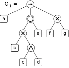
Figure 3shows an example of a process tree modelQ1that contains 7 activities and 5 operators.

Thisprocesstreecontainsasequenceoperator(→)asarootnode,i.e.,itsbrancheswillbeexecutedfrom

lefttoright.Hence,thefirstactivitytobeexecutedwillbea.Then,thereisaloopoperator( ).Itsleftmost

branchrepresentthe“do”partoftheloop,itwillbeexecutedatleastonceandtheloop

executionwillalwaysstartsandendswithit.Inthiscase,thereisanexclusivechoiceoperator(×) inthe

leftmostbranch,indicatingthateithertheactivitybortheparallel(∧)activitiescanddwillbe executed.

Therightmostbranchoftheloopoperator( )representsthe“redo”partoftheloop,which

inthiscasecontainsonlytheactivitye. Theprocessendswithaexclusivechoiceoperator(×)that

indicatesthefinalactivitywillbe f org.

II

I

a

b

c d

e f g

III

Q =₁

(6)

3.4.ConfigurableProcessTree

Representing configurable process models as process trees has been addressed by [9,10]. We have

slightlyredefinedthedefinition ofconfigurable processtrees described bythemon ourproposed

framework, in order to allow greater flexibility and expressiveness in theconfigurable nodes. A

configurable processtree (CPT)representsafamilyof processmodels [23]. All processesofa family

share the same tree topology, while differences are handled using configurable nodes. Applying a

particularconfigurationtotheseconfigurable nodesproducesavariantoftheconfigurableprocess

model,aderivedprocessmodel. Aconfigurablenodecanbesettoenable(orallow),hideorblock.

Enable(allow)meansthenodeisenabledtobevisited,hidemeansthenodeistobeskippedover,and

blockmeansthenodecannotbereached. Thefoundationofconfigurableprocesstreesisdescribed in

[10],andalsoappliedin[9].

Definition4(Processtreeconfigurators). =_{H,B,E}isthesetofprocesstreeconfigurators,and

× = {{H},{B},{E},{H,B},{H,E},{B,E},{H,B,E}} is the set of all subsets of the process tree

configurators,where:

• H:hidea node. It makes a node unobservable, replacing it by aτnode.

• B: blocka node. It makes the leading path to this node unreachable. When blocking a node, several cases might occur; details can be found in [18].

• E:enablea node. It essentially allows a node to be performed, either an operator or an activity, so that it behaves normally.

Definition5(Configurableprocesstree).AconfigurableprocesstreeQα₌₍_Q,_α₎_is_comprised

of a process tree Q with N(Q) nodes, and a partial configuration function α : N(Q) 9 ×

α α

definingaconfigurationsetforsomenodes.N(Q)_⊆N(Q)isthesetofconfigurablenodes,i.e.,Nα₍_Qα₎₌

domain(α).Forthesakeofclarity,letusassumeanorderingamongtheconfigurable

nodes, i.e., n1,n2, . . . ,n_|Nα₍_Qα₎_|. C(Qα) is the set of all possible configurationsof Qα, i.e., C(Qα) =

{hc1,c2, . . . ,c_|Nα₍_Qα₎_|i|c_i∈α(n_i)}.

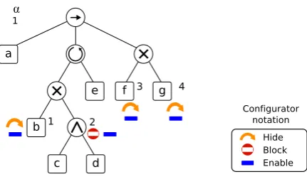
Figure 4is an example of a configurable process treeQα

1that contains 4 configurable nodes, listed

from1to4. Configurablenodes1,3and4canbeeitherhiddenorenabled,whereastheconfigurable

node2canbeeitherblockedorenabled.

II

I

a

b

c d

e f g

II

1 2

3 4

1⍺

Configurator notation

Hide Block Enable

Figure 4.Example of a configurable process tree containing 4 configurable nodes.

It is possible to apply a configuration to a configurable process tree in order to obtain a process

(7)

Definition 6(Derived process tree). LetQα _{be a configurable process tree, and let}_c _∈ _C₍_Qα₎_{be a}

possibleconfiguration.derive(Qα_,_c₎₌_Q

cisthefunctionthatgeneratesaderivedprocesstreeQcfromQα

byapplyingtheconfigurationc,usingtherulesappliedin[18].

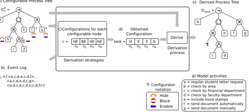
Figure 5 presents a running example of the execution of the derivation framework shown in Figure 2. A configurable process tree and an event log are the inputs, depicted in a) and b),

respectively. The implemented derivation strategies use a common data structure to represent all

thefeasibleconfigurationsforallconfigurablenodes,showninc). Eachderivationstrategyallows to

obtain a configuration, shown in d), which is then used to derive a process tree, shown in e).

Figure5 also depicts thenotation for theprocess treeconfigurators and themodel activities in f)and

g),respectively. II III a b c d

e f g

III

Configurable Process Tree

Configurations for each configurable node

HE BE HE HE, , , , c = 1 {<a,c,d,e,c,d,f>, <a,c,d,e,d,c,g>, <a,d,c,e,c,d,e,c,d,f>} Event Log

Derived Process Tree

Obtained Configuration II III a c d

e f g

II

H E E E

best = Configurator notation Hide Block Enable 1 2 3 4

τ

L = 1

a b c d e f g = = = = = = =

regular student letter request check by area

check by financial department check by faculty department include more stamps send document automatically send document manually Derivation strategies a) c) g) f) b) e) d) Derive Model activities Derivation process

Q =⍺1 Q =best

n n2 n3 n4 n1 n2 n3 n4

Figure 5.Running example that illustrates the derivation framework. A configurable process tree and and event log, shown in a) and b), are the inputs. The internal representation of a configuration used by the three strategies is represented in c). The obtained configuration is shown in d). Finally, the output, a derived process tree is shown in e).

3.5.QualityofaDerivedProcessTree

Several configurations can be applied to a configurable process tree. In order to asses the

qualityof a derived processtree to represent theobserved behavior in an event log,a qualitymetric

must be defined. Quality is usually measured considering a trade-off among the following four

quality criteria: fitness, precision, generalization, and simplicity [8,20,24]. Conformance checking is a

subdisciplineofprocessminingthatallows tocomparethebehavior allowedbya processmodelwith

thebehavior recorded in an event log to find commonalities and discrepancies, and also to compute

metricsforeachofthefourqualitycriteria[24].

Definition 7(Conformance). Let Qbe a process tree and let Lbe an event log. Letf,p,g,sbe the fitness, precision, generalization, and simplicity metrics as defined in [18] with a range [0,1], being

1 the target value, and letW = (wf,wp,wg,ws) be the weights given to each metric, respectively.

Conformanceis defined as:

conformance(Q,L,W) = f(Q,L)·wf +p(Q,L)·wp+g(Q,L)·wg+s(Q,L)·ws

(8)

In this article, we have defined the conformance metric based on [18] and used the corresponding

implementationtoevaluatethequalityofagivenprocesstree.However,theproposedframeworkis

genericandindependentoftheconformancemetricused.

An optimal configuration is the one that allows to obtain a derived process tree that better

representsagiveneventlog,e.g.hasthebestconformancevalue.

Definition8(Optimalconfiguration).LetQα_be_a_configurable_process_tree,_let_L_be_an_event_log,_and

letWbetheweightsofthequalitymetrics.Aconfigurationc∈ C(Qα₎_is_an_optimal_{configuration}_if _and

only if there is not another configuration c0 ∈ C(Qα₎ _such _that _conformance₍_derive₍_Qα_, _c0₎_, _L, _W₎ _>

conformance(derive(Qα_,_c₎_,_L,_W₎_.

Our goal is to automatically obtain a configuration to derive a process tree from a configurable

processtreethatmaximizestheconformancefunctionforagiveneventlog. Toaccomplishthisgoal,

wehaveimplementedthreestrategies,whicharedetailedinthenextsection.

4. Methodology

As part of the proposed framework, we have designed three different derivation strategies that

areable to find a suitable configuration in order to derive a process tree. The first strategy is based

on an exhaustive approach, guaranteeing to find an optimal configuration. The other two strategies

arebased on heuristicsthat find a configurationthat allows to derive a reasonably good processtree

ina fastertime. Each of these strategies isdescribed hereafter. Noticethat the approach proposedin

this articleis different to theone proposed in[18]. In[18], theinput is a collection of event logs and

theoutput is a configurable process model. In our case, the input is an alreadyexisting configurable

process model and an event log. The output is a feasible configuration of the input configurable

processmodel, so as the derived process model obtained with such a configuration better represents

theinputeventlog.

4.1.Obtainingaconfigurationbasedontheexhaustivestrategy

The first strategy in the proposed framework is the exhaustive strategy, whose relevance is that

itensuresobtainingthebestconfigurationamongallpossibleones.Ingeneral,anexhaustivestrategy isa

brute-forcemethodtoaprobleminvolvingthesearchforasolutionamongallpossibleones,e.g., those

obtained from combinatorial objects, such as permutations or combinations. In this case, for a

configurableprocesstreeQα_,_we_analyze_all _possible_{configurations}_that_belong_to_C₍_Qα₎_._Algorithm ₁

presentstheexhaustivestrategy,whichcanbedescribedasfollows:

• Generate the set of all possible configurations, C(Qα₎_{, in a systematic manner, using the}

Cartesian product of the configuration sets for all configurable nodes.

• Loop over all configurations. At each iteration, the function derive(Qα_,c)_{is used to obtain a}

derived modelmfrom theCPT Qα_{, given the configuration}_c.

• The modelmis evaluated using theconformancefunction defined inEquation 1.

• All potential configurations are evaluated, keeping track of the best solution found.

• After all configurations have been processed, the algorithm returns the configuration with the

highest conformance.

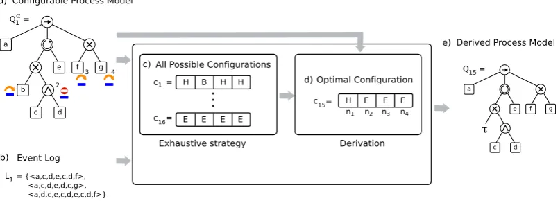
Figure 6 presents an illustrative example of the exhaustive strategy. Given the CPT Qα

1 and

thelog L1,shown ina) andb), theframeworkfindsthebestconfigurationandthecorresponding

derived process tree. The CPTQα

1, shown in a), has 4 configurable nodes, where the activity node

(9)

orE, and the activity nodegcan be eitherHorE. The set of configurationsC(Qα₎_{contains 2}4 ₌₁₆

differentconfigurations.Theframeworkcheckseveryconfigurationc∈C(Qα),showninc).Among

allpossiblefeasibleconfigurations,thealgorithmselectsc15 asthebestconfiguration,shown ind).

Once the best configuration is obtained, the framework applies it to theCPT Q α

1to derive the process

treeQ15,shownine).

II

III a

b

c d

e f g

II

L = {<a,c,d,e,c,d,f>, <a,c,d,e,d,c,g>, <a,d,c,e,c,d,e,c,d,f>}

Event Log

2

3 4 All Possible Configurations

H B H H

c = 1

E E E E

16

..

.

1

Derived Process Model

Optimal Configuration

H E E E

Exhaustive strategy

e)

d)

Derivation

II

III a

c d e f g II

τ Q =₁

Configurable Process Model a)

b)

Q =₁₅

15

c)

⍺

1

n n2 n3 n4

c =

Figure 6. Overview of the exhaustive strategy to derive a process tree. The algorithm generates all possible configurations, in order to find an optimal configuration. This configuration is used to obtain an optimal derived process tree.

Algorithm 1Obtain a configuration based on the exhaustive strategy

1: procedureEXHAUSTIVE(LOGL, CPTQα, WEIGHTSW)

2: best←null

3: C(Qα₎_←_{CartesianProduct}₍_α₍_n

1),α(n2), . . . ,α(n_|_Nα₍_Qα₎_|))

4: for allc∈C(Qα)do 5: m←derive(Qα_,_c₎

6: ifconformance(m,L,W)>conformance(derive(Qα_,_best₎_,_L,_W₎_then

7: best←c

8: end if

9: end for

10: returnbest

11: end procedure

4.2.Obtainingaconfigurationbasedonthegeneticstrategy

The exhaustive strategy requires a long time to find an optimal solution. Motivated to find

a solution in less computing time, we have designed a second strategy to find a reasonable

good configuration, based on a genetic evolutionary approach. Genetic algorithms (GA) are

search algorithms that imitate the process of natural selection in nature, belonging to the class of

evolutionary algorithms [25–27]. In this subsection, we present a GA approach to find a suitable

configuration for a CPT model given a specific event log. The elements that define a GA are:

representation of individuals, initialization, selection, crossover, mutation, and termination condition.

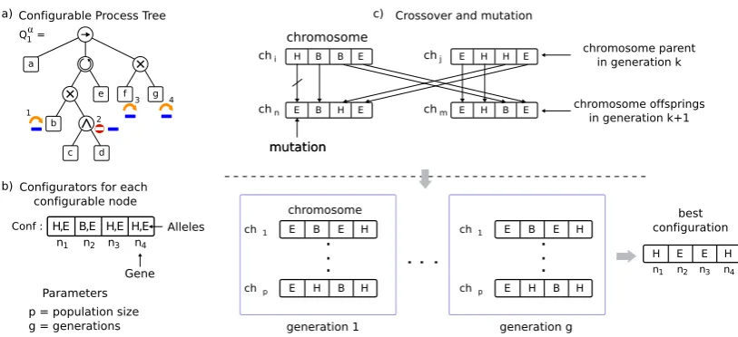
Next, we present the setting of each of these elements in our configuration scenario. Figure 7

illustratesthesemainelements.

(10)

value of a gene is called an allele. In our case, a chromosome represents a configuration

c ∈ C(Qα₎_{, see}_{Figure 7}_{b), where each gene}_c

i corresponds to a configurable nodeni, and an

allele is a configurator (B,H, orE) assigned to that particular configurable node,ci ∈α(ni), for

alli∈1, . . . ,|Nα₍_Qα₎_|_.

• Initialization : An initial population is generated randomly, where each individual represents

a randomly created configuration c using valid alleles, i.e., ci ∈ α(ni). Population size is a

parameter that determines the number of individuals in the first generation [28].

• Selection : In each generation, the best candidates are selected to move forward to the next generation, and some of them are also selected to be recombined. Each individual is evaluated

using the conformance function1that evaluates the quality of achromosometo either be selected

for the next generation or to be discarded. We refer to [25] to illustrate different selection strategies.

• Crossover : The crossover operation combines two parent chromosomes in order to generate

two offspring chromosomes, as it is shown inFigure 7c). Given two chromosomesaandband

a cutting point 1≤i< |Nα₍_Qα₎_|_{, the offspring chromosomes are}_h_a

1, . . . ,ai,bi+1, . . . ,b|Nα₍_Qα₎_|i

and hb1, . . . ,bi,ai+1, . . . ,a_|Nα₍_Qα₎_|i. Notice that, the proposed chromosome representation

combined with the defined crossover operation produce only valid solutions, i.e. the

offspring chromosomes are always valid configurations, according to the definitions presented insubsection 3.4.

• Mutation : A mutation produces a random change in one of the genes of the chromosome. In order not to produce spurious chromosomes, the mutation of a gene is restricted to the valid

alleles of the gene, i.e.,ci ∈α(ni), whereiis the mutated gene.

• Termination conditions : The most common alternatives forGAto terminate are: an upper limit for the number of generations, an upper limit for the conformance function (1 in our case), when the likelihood of achieving significant improvements in the next generation is very low, or when a given number of generation does not get any improvements [25].

Algorithm 2 describes the basic GA strategy. The main inputs are a configurable process

model and an event log. The initialization of chromosomes is made in initialPopulation(), then

all chromosomes of the initial population pop are evaluated using the conformance function in

bestIndividual(pop), in order to obtain the best individual. The population evolves over several

generations until a termination condition is reached. In each generation, the algorithm selects

qualified individuals through elitism in selectParents(pop). Later, the function crossover(parents)

recombinespairsof parents to createnew individuals, in thisway, a new populationpop’is obtained.

Mutation is then applied randomly to this new population, obtaining the new generation pop”. The

bestindividual in the population pop” isthen comparedto the best configurationobtained so far. At

the end, the algorithm returns the best individual (configuration) obtained using this evolutionary

approach. For the sake of generality, Algorithm 2 describes the most generic GA strategy. More

sophisticated techniques for each step of the algorithm are also possible (e.g., tournament, elitism,

amongothers).Pleasereferto[18,25]formoredetails.

1 _{In GA theory, the function that evaluates the quality of a chromosome is called}_fitness_{. This fitness function does not}

correspond to the fitness function presented insubsection 3.5, but to the conformance function. Therefore and for the sake

(11)

mutation II III a b c d

e f g

II

Configurators for each configurable node

HE B E H E H E, , , ,

Conf :

Crossover and mutation

1

2

3 4

chromosome

E B E H

ch 1

E H B H

chp

.

generation 1

E H H E

chj

H B B E

ch i

E H B E

chm

E B H E

chn

mutation

chromosome parent in generation k

chromosome offsprings in generation k+1

Gene

p = population size g = generations

E B E H

ch 1

E H B H

chp

.

best configuration Parameters

.

c) a) b)

H E E H

Alleles

Q =₁⍺

1

n n2 n3 n4

1

n n2 n3 n4

chromosome

generation g

Figure 7. Overview of the genetic strategy to derive a process tree. The internal configuration representation allows this evolutionary algorithm to use crossover and mutation operations to generate new candidate configurations to be assessed.

Algorithm 2Obtain a configuration based on the genetic strategy

1: procedureGENETIC(LOGL, CPTQα_{, W}_EIGHTS_W₎ 2: pop←initialPopulation(Qff)

3: best←bestIndividual(pop)

4: whilenot TerminationCondition()do

5: parents←selectParents(pop) 6: pop0←crossover(parents) 7: pop00 ←mutate(pop0)

8: m←derive(Qα,bestIndividual(pop00))

9: ifconformance(m,L,W)>conformance(derive(Qα_,_best₎_,_L,_W₎_then 10: best←bestIndividual(pop00)

11: end if

12: end while

13: returnbest

4.3.Obtainingaconfigurationbasedonthegreedystrategy

The above described evolutionary strategy is able to find a good configuration (potentially an

optimal one [25]) in less timethan the exhaustive strategy, but it is still time consuming. In order to

reducethetimeevenmore,butatthesametimetobe abletofindareasonablygoodconfiguration,we

presentathirdstrategy,basedonagreedyheuristic. Agreedystrategyisaheuristicsearchthatcreatesa

feasible solution incrementally, always making thechoice that looks bestat the moment of making a

local choice. Sometimes these local choices lead to a global optimal solution [29]. Depending onthe

problem and search space, this strategy does not result in finding one of the optimal solutions,

however for many problems they provide a close to optimal solution (even an optimal one) in a

reasonablecomputingtime.

Greedy algorithms usually divide the problem in small sub-problems; each sub-problem is then

solved independently and in an incremental fashion. In our case, we can take subtrees from the

configurable process tree and process each of them independently, and make good localchoices in the

hopethat they result in an optimalsolution when weapply all these localconfiguration choices to the

(12)

In a configurable process tree, two (or more) configurable nodes aredependentif one of them is

underorabovetheotheroneinatreebranchoriftheybothhaveacommonancestorthatisa

operator. Ifso, theconfigurationofone ofthese nodesmight affecttheconfigurationof theotherone.

On the other hand, a configurable node is independent if it is not dependent of any other configurable

node.

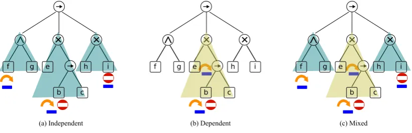
We can identify three scenarios in a configurable process tree depending on the dependency

among its configurable nodes. The configurable process tree can have only independent configurable

nodes, as shown in Figure 8 (a); it can have only dependent configurable nodes, as shownin

Figure 8 (b); or it can combine both independent and dependent configurable nodes, as shown in Figure8(c).

(b) Dependent

(a) Independent (c) Mixed

II

III

II III II II

II II

III

f g e h i

c b

f g e h i

c b

f g e h i

c b

Figure 8.Different configurable node dependencies.

Algorithm3describes the proposed greedy strategy, which consists of the following steps:

• The configurable process tree is traversed to obtain a sorted list of all configurable nodes. A

hierarchical order is achieved by applying the following rules:

– Dependentconfigurable nodes have a higher priority thanindependentconfigurable nodes.

– Among configurable nodes of the same type (dependentorindependentconfigurable nodes),

a deeper configurable node has a higher priority.

– Among configurable nodes in the same level, an operator node has a higher priority than

an activity node; otherwise, they are sorted from left to right.

• Every configurable node is then processed accordingly to its priority. For each configurable

node, a subtree and a sublog are obtained to compute the local conformance:

– To obtain a subtree for a configurable node, a new root has to be considered. If a

configurable node is an activity node, the new root is its direct parent, so that a subtree always has an operator as a root; otherwise, if it is an operator node, the new root is the own operator node. If the configurable node has some ancestor that is a loop operator, then the new root is the loop operator ancestor that is close to the original root. Such a new subtree might contain other pending configurable nodes; they are temporarily set to

τin order to postpone any decision about their configuration.

– To obtain a sublog, we get the projection of the event log on the set of activities contained

(13)

• For the selected configurable node, all possible configurators are evaluated, obtaining different derived process subtrees. The local conformance between each of those process subtrees and the event sublog is computed. The best configurator is saved and then set in the best configuration for the original configurable process tree.

• At the end, the best configuration for the whole configurable process tree is returned.

Figure 9illustrates the greedy strategy to find a configuration for the configurable process tree Qα

1. The derivation process is shown on the right part of the figure for two logs,L1andL2, where, for

everyconfigurablenode,thebestconfiguratorisselectedamongallfeasibleconfigurationsforeach

configurablenode. First,theorderinwhichtheconfigurablenodeswillbeprocessedisdecided. n1

andn2aredependentnodesbecausetheyhaveacommonancestorthatisa operator.Meanwhile,

n3and n4areindependentnodes.Hence,n1andn2havea higherprioritythann3and n4.Sincen2 isan

operatornode,ithasahigherprioritythann1.n3andn4arebothactivitynodes,sotheyare prioritized

fromleft (n3) toright(n4).Therefore,theorder isn2,n1,n3,n4,regardlessoftheevent log thatwillbe

considered. For the event log L1,the algorithm startsfrom the deeper node n2. n1is set to τ and all

possibleconfigurators(BandE)forn2arethenevaluated,consideringthesubtreethathas asarootthe

loopoperator that isan ancestor of n2,and thesublog obtained projectingthe original log L1on the

activitiescontainedinthesubtree:c,d,e.Thebestconfigurationforn2isE.Later,havingtheconfiguration

ofn2,inasimilarwayn1isanalyzedandconfiguredtoE.Afterwards,n4issettoτ whilen3isconfigured

toE.Finally,oncen3isalreadyconfigured,thelastnoden4isconfiguredtoH. Thefinalconfiguration

forL1isthen obtained,andrepresented asthebestconfiguration. For theevent log L2, thealgorithm

proceedsinasimilarway.NoticethatsincethelogL2containsfeweractivities

that the configurable process treeQα

1, the projection of the activities contained in the subtrees creates

verysimplesublogs,even an emptyevent log,suchastheobtainedwhen processingtheconfigurable

node n2. The best configurationin this caseconsiders to blockthe configurable node n2 and hide the

configurablenoden4,illustratinghowthealgorithmadaptstodifferentscenarios. Asaresult,Q1is

the derived process tree fromQα

1andL1, andQ2is the derived process tree fromQ α1andL2.

II

III

a

b

c d

e f g

II

Configurators for each configurable node

HE BE HE HE, , , , c =

1 2

3 4

E B E H

b L =

{<a,b,f>} {<a,c,d,e,c,d,f>, <a,c,d,e,d,c,g>, <a,d,c,e,c,d,e,c,d,f>} Event Log II a b e f II _τ II III c d e f II g τ subTree

subLog{< >}

e II subLog{<b>} subTree subTree subLog{<f>} τ II f subTree subLog{<f>} g best configuration Derived Process Tree Event Log III c d e II τ subTree subLog {<c,d,e,c,d> <c,d,e,d,c> <d,c,e,c,d,e,c,d>} b e II subTree subLog {<c,d,e,c,d> <c,d,e,d,c> <d,c,e,c,d,e,c,d>} III c d

H E E E

II a e f II II f subTree subLog{<f> < > <f>} τ II f subTree subLog{<f> <g> <f>} E g

Derived Process Tree

best configuration III c d τ 2 1 Q = Q = Q =₁⍺

1

n n2 n3 n4

1

n n2 n3 n4 1

2 2

c E c1 H c3 E c4

H 4 c 3 c E 1 c E 2 c B

(14)

Algorithm 3Obtaining a configuration based on the greedy strategy

1: procedureGREEDY(LOGL, CPTQα_{, W}_EIGHTS_W)

2: configurableNodeList←getPrioritizedConfigurableNodes(Qff) 3: bestConfiguration←emptyConfiguration()

4: for allcn∈configurableNodeListdo

5: sQα_←_{getSubTreeFromConfigurableNode}₍_Qα_,_cn₎ 6: activityList←getActivityNodes(sQα₎

7: sL←LactivityList

8: best←null

9: for allcon f igurator∈α(cn)do

10: m←derive(sQα,con f igurator)

11: ifconformance(m,sL,W)>conformance(derive(sQα_,_best₎_,_sL,_W₎_then 12: best←con f igurator

13: end if

14: end for

15: bestConfigurationcn←best

16: end for

17: returnbestConfiguration

19:

20: proceduregetSubTreeFromCon f igurableNode(CPTQα_{, C}_ONFIGURABLE_N_ODE_cn) 21: ifIsActivityNode(Qα_,_cn₎_then

22: nodeRoot←getParent(Qα_,_cn₎ 23: else ifIsOperatorNode(Qα_,_cn₎_then 24: nodeRoot←cn

25: end if

26: for alln∈ Ancestors(Qα_,_nodeRoot₎_do 27: ifIsLoopOperatorNode(Qα_,_n₎_then

28: nodeRoot←n

29: end if

30: end for

31: sQα_←_getSubTree₍_Qα_,_nodeRoot₎

32: for alln∈ Descendants(sQα_,_nodeRoot₎_do

33: ifn6=cn && IsCon f igurableNode(sQα_,_n₎_then

34: n←τ

35: end if

36: end for

37: returnsQff

5. ResultandDiscussion

The proposed strategies have been implemented and evaluated in two different scenarios. In

this section, we first describe how the framework has been implemented (see subsection 5.1). Then,

we describe the two scenarios considered: a realistic scenario based on the adoption of a higher

educational ERP system by some universities (see subsection 5.2), and a scenario that representsa

real-life registration process [30], which is executed on a daily basis by Dutch municipalities(see

subsection 5.3). Afterwards, in subsection 5.4, we analyze the performance of the proposed

strategies on a set of controlled experiments created for testing the performance of the strategies

(15)

5.1.Implementation

We have implemented the three strategies, exhaustive, genetic and greedy, as three plug-ins

of the ProM process mining framework2, within the ConfigurableProcesses package. The genetic

evolutionary strategy is implemented using JGAP, a Java library for GA; this flexible library fits in

our genetic evolutionary approach. All experiments have been performed in a laptop with an Intel

Corei5CPUat2,7GHz,8GBRAM,runningOSXElCapitan64bits.

5.2.Educationalscenario

Educational institutions such as universities are spread along cities in a country with the purpose

of granting academic degrees in various subjects. When the owner of a network of universities

decidestostandardizethehighereducationalERPsystemtobeusedforalltheuniversitiesbelongingto

thenetwork,thefirststepistoknowhowsuitablethesoftwareisforeachuniversity.

The ERP system provides support for different processes, and it can be configured to suit how

eachprocess isexecuted in theuniversity where it will be installed. The diversity of processvariants

the ERP supports can be represented through a configurable process model. The decisions that are

made to adapt the software to the way the process is executed in each university corresponds to

the configuration that allows to generate a derived process model specific for each university. The

derived process model will probably not be exactly the same as the process model that represents

howthe processiscurrentlyexecuted,but it willbe theclosest processvariantthe softwareis ableto

support.

If a university is currently running the process using other software, we can assume an event log

iscurrentlyrecordinghoweachprocessisbeingexecuted.

The framework proposed in this article takes as input the configurable process model that

representsthe different parameterizations provided by the ERP system for theprocess and the event

logthatrepresentsthecurrent executionoftheprocessina university. Based onthem,theframework

generates a derived process model that representshow the process could be run in the future using

theERPsystem.

Academicplanningprocess

Beyond their organizational structure, universities share some common processes, such as

planning academic courses. The planning of academic courses in a university is a complex

processdue to several factors such as government regulations, internal policies, dynamic changes of

knowledge in certain domains, economic and human resources, among others. In this process, both

administrativepersonnel and facultymembers,sometimesfrom differentdepartments,areinvolvedin

each stage of the process. This process, in general, considers some similar stages across universities

such as course planning, student assistant planning, thesis planning, among others. To deal with its

complexity,it canbe modeled at ahigh-level. Figure 10depicts a generalprocessmodel thatincludes

sub-processesthatgroupcommonactivitiesintheacademicplanningprocess.

We have used this process model as a reference process model for three different universities

located along a country. For the sake of simplicity, we call them: Northern University, Central

University, and Southern University, according to their location in the country. Each university

executes a different process variant of the reference model according to its policies, regulations,

socio-demographic characteristics, and geographic needs. For example, the Northern University isa

low-income university, so there are some coursesthat do nothave student assistants, whereas inthe

othertwo high-income universitiesthere is more thanone student assistant in some courses.

(16)

start

Academic planning start

Academic planning

end end

Prepare academic

program

Update academic

program

Publish academic

program

Student assistant planning

Thesis planning

Adjust academic

program

Figure 10.General model of the academic planning process of a university. It includes parallel flows that contain sub-processes.

The SouthernUniversity doesnot havea proper internal informationsystem, so selecting student

assistantsisamanualtask.

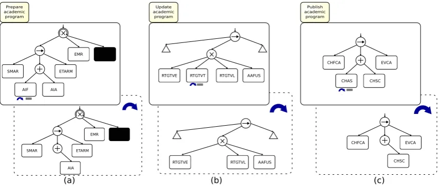
The configurable process tree contains 70 activities, grouped in the 8 sub-processes shown inFigure10,and9configurablenodesthathavemixeddependencies.Theconfigurableprocessmodelis

considerablylarge,making it impractical to showit completely. To illustrate howthe configurationis

performed, Figure 11 shows a scheme of the configuration process. The upper boxes represent

configurable process trees for three different sub-processes of the process reference model. The

lower process trees, inside the dash line boxes, are derived process trees where the corresponding

configurablenodeshavebeenconfiguredashide.

Publish academic program Update

academic program Prepare

academic program

SMAR

AIA ETARM

EMR

RTGTVE RTGTVL AAFUS

CHFCA

CHSC EVCA SMAR

AIF AIA ETARM

EMR

RTGTVE RTGTVT RTGTVL AAFUS

CHFCA

CHAS CHSC EVCA

(a) (b) (c)

Figure 11.General idea of process model derivation for three different configurable sub-processes.

Having a reference process model, whose overall view is shown inFigure 10, and an academic

planningevent log per university, it was possible to derive a process model for each university. We

appliedtheproposedexhaustive,genetic,and greedystrategiestothethree cases. Theresultsareshown

inTable 1,includingfitness, precision,and theconformancemetric,calculated as90%fitnessand 10% precision.

It is possible to observe inTable 1that bothNorthernUniversity andCentralUniversity have a

highconformance,and alsoa highfitness. Wecanassertthatbothuniversitieshavea highpercentage

of commonality with the configurable process model. However, that is not the case for Southern

University, which has a lower conformance and a lower fitness. One of the reasons for this is the

(17)

in the reference model. A decision maker would probably decide the ERP system that is desired to

acquireisnotsuitableforthisuniversity.

Table 1.Comparison of the proposed strategies for the three universities.

Northern Central Southern

fitness precision conformance fitness precision conformance fitness precision conformance

Exhaustive 0.981 0.398 0.922 0.986 0.510 0.939 0.690 0.510 0.672

Genetic 0.981 0.398 0.922 0.986 0.510 0.939 0.690 0.510 0.672

Greedy 0.981 0.370 0.920 0.986 0.500 0.938 0.690 0.500 0.671

Table 1shows that all three strategies obtained process trees with the same fitness. However, the

greedystrategy obtained a process tree with a lower precision. Taking theNorthern University asan

example, a qualitative analysis between the process tree obtained by the exhaustive strategy and the

greedy strategy suggests that the exhaustive strategy finds a configuration of the model where the

activity Assign Classroom Automatically (ACA) is always performed (as observed in the event log),

while the greedy strategy finds a configuration of the model where the activity ACA can either be

performedorskipped(thatwasneverobservedintheeventlog),obtainingalowerprecision.

The performance of the three strategies is depicted inFigure 12. It is possible to observe that the

time required by the exhaustive strategy is considerably higher than the time required by the genetic

and greedy strategies. Moreover, the greedy approach was able to obtain a derived process model

in seconds whereas the other two algorithms required minutes and even hours. The time required

in the case of the Southern University is higher due to the alignment technique used to obtain the

conformancemetric. As itwas mentioned before, at theSouthernUniversity,manyactivities arebeing

executed that are not found in the reference model; in those cases, the alignment technique takes

longer[31].

Time

(hh

:mm)

0:00 0:30 01:00 01:30 02:00 02:30 03:00

Exhaustive Genetic Greedy

Northern

Central Southern

Figure 12.Benchmarking of the performance of the three strategies.

In conclusion, thegreedystrategy is able to obtain in a short time a derived process model that has

aquitegoodconformance,incomparisontotheconformanceobtainedwiththeothertwostrategies.

5.3.Real-lifeexperiments

In order to evaluate the performance of the techniques on real-life data, we apply all three

strategiesonareal-lifedataset. Thedatausedcontainseventdatafromthebuildingpermitsprocessof

five Dutch municipalities [17,32]. There are five event logs, each describing a different process

variant,which were extracted from the IT systemsof the corresponding municipality. Thesame data

hasbeen usedto evaluatetheperformance of configurableprocessdiscovery of theEvolutionaryTree

Miner (ETM) [18, pages 250 and 251]. In this experiment, we create some CPTs based on two of the

(18)

the CPTs to come to the best solution they can achieve. We then compare these results with the results

obtainedbytheETMonthesamedataset.

We use CPTs based on the models discovered by the ETM on this dataset, which are shown in Figure 13. Figure 14 shows the two CPTs created based on the model shown in Figure 13a. The CPT in Figure 14a has two configurable nodes while the CPT in Figure 14b has eight configurable

nodes, all randomly chosen. Noticethat we could not create a CPT similar to Figure 13a because we

are not considering the downgrade operator used in [18]. Figure 15 shows the three CPTs created

basedon themodel shown inFigure 13b. TheCPT inFigure 15a isequivalentto theone shown in

Figure 13b. The CPT in Figure 15b has six configurable nodes while the model in Figure 15c has

twelve configurable nodes, all randomly chosen. All configurable nodes can be set to enable (or

allow),hide orblock. Wealloweachofthethreestrategiestoconfigureall modelsto cometothebest

solutiontheycanachieve. Wethen comparethese resultswiththeresultsobtained bytheETM onthe

samedataset.

∨

×

770 765 ∨

→ 550 × τ ∨ × ∨ → 600 610 740 770 630 560 755 × →

550_1 755 766 590 × 540 ∧ 540 770 ∨ 630 730 [∧,-,-,-,-]

[←,B,-,→,→]

[∧,-,→,-,-]

[-,→,←,→,→]

[→,→,∧,×,∧]

[ Monday 26th_{May, 2014 at 11:25 –}_??_{pages – version 0.2 ]}

(a)ETM - Approach 3

→

×

630 540 _→

×

770 540 _→

630 730 755 ×

τ 540 →

550 560 630 730 → 630 730 × τ 765 × τ 770 [-,H,-,-,-]

[ Sunday 25th_{May, 2014 at 13:41 –}_??_{pages – version 0.2 ]}

(b)ETM - Approach 4

Figure 13.Process trees originally discovered by the ETM on the WABO event logs.

∨

×

770 765 ∨

→ 550 × τ ∨ × ∨ → 600 610 740 770 630 560 755 × →

550_1 755 766 590 × 540 ∧ 540 770 ∨ 630 730

(a)CPT 3-A, contains 2 configurable nodes

∨

×

770 765 _∨

→ 550 × τ _∨ × ∨ → 600 610 740 770 630 560 755 × →

550_1 755 766 590 × 540 _∧ 540 770 ∨ 630 730

(b)CPT 3-B, contains 8 configurable nodes

Figure 14.CPTs based on the model discovered by the ETM Approach 3.

The results of the experiments with the CPTs created based on the model discovered by the

ETMApproach3areshowninTable 2 andTable 3.Table 4,Table 5 andTable 6 showtheresultsofthe

experimentswith theCPTscreatedbased onthemodeldiscoveredbytheETMApproach 4. Alltables

(19)

→

×

630 540 →

×

770 540 →

630 730 755

×

τ 540 →

550 560 630 730

→

630 730

×

τ 765

×

τ 770

(a)CPT 4-A, contains 1 configurable node

→

×

630 540 →

×

770 540 →

630 730 755

×

τ 540 →

550 560 630 730

→

630 730

×

τ 765

×

τ 770

(b)CPT 4-B, contains 6 configurable nodes

→

×

630 540 →

×

770 540 →

630 730 755

×

τ 540 →

550 560 630 730

→

630 730

×

τ 765

×

τ 770

(c)CPT 4-C, contains 12 configurable nodes

Figure 15.CPTs based on the model discovered by the ETM Approach 4.

Table 2.Results for CPT 3-A and the event logs corresponding to the five process variants

Variant 1 Variant 2 Variant 3 Variant 4 Variant 5

f p fpc f p fpc f p fpc f p fpc f p fpc

Exhaustive 0.941 0.745 0.921 0.962 0.768 0.943 0.936 0.646 0.907 0.985 0.751 0.962 0.950 0.797 0.935

Genetic 0.941 0.745 0.921 0.962 0.768 0.943 0.936 0.646 0.907 0.985 0.751 0.962 0.950 0.797 0.935

Greedy 0.878 0.720 0.862 0.908 0.802 0.897 0.855 0.635 0.833 0.973 0.748 0.951 0.907 0.753 0.892

ETM 0.948 0.842 0.937 0.948 0.979 0.951 0.927 0.729 0.907 0.984 0.917 0.977 0.957 0.909 0.952

f = fitness, p = precision, fpc = conformance

Table 3.Results for CPT 3-B and the event logs corresponding to the five process variants

Exhaustive 0.941 0.745 0.921 0.962 0.768 0.943 0.936 0.646 0.907 0.985 0.751 0.962 0.950 0.797 0.935

Genetic 0.941 0.745 0.921 0.962 0.768 0.943 0.936 0.646 0.907 0.985 0.751 0.962 0.950 0.797 0.935

Greedy 0.878 0.720 0.862 0.908 0.802 0.897 0.855 0.635 0.833 0.973 0.748 0.951 0.907 0.753 0.892

ETM 0.948 0.842 0.937 0.948 0.979 0.951 0.927 0.729 0.907 0.984 0.917 0.977 0.957 0.909 0.952

Table 4.Results for CPT 4-A and the event logs corresponding to the five process variants

Exhaustive 0.958 0.730 0.935 0.962 0.912 0.957 0.945 0.648 0.915 0.993 0.849 0.979 0.954 0.931 0.952

Genetic 0.958 0.730 0.935 0.962 0.912 0.957 0.945 0.648 0.915 0.993 0.849 0.979 0.954 0.931 0.952

Greedy 0.944 0.737 0.923 0.960 0.789 0.943 0.934 0.644 0.905 0.996 0.750 0.971 0.943 0.781 0.927

ETM 0.948 0.842 0.937 0.948 0.979 0.951 0.927 0.729 0.907 0.984 0.917 0.977 0.957 0.909 0.952

Table 5.Results for CPT 4-B and the event logs corresponding to the five process variants

Exhaustive 0.911 0.951 0.915 0.980 0.962 0.978 0.948 0.894 0.943 0.986 0.978 0.985 0.949 0.975 0.952

Genetic 0.911 0.951 0.915 0.980 0.962 0.978 0.948 0.894 0.943 0.986 0.978 0.985 0.949 0.975 0.952

Greedy 0.911 0.951 0.915 0.970 0.970 0.970 0.938 0.911 0.935 0.985 0.899 0.976 0.947 0.976 0.950

ETM 0.913 0.921 0.914 0.980 0.962 0.978 0.948 0.894 0.943 0.986 0.978 0.985 0.949 0.975 0.952

It can be observed that in all cases the different strategies obtain good results. Since the

exhaustive strategy always obtains thebest possible result, we can highlightthat the genetic strategy

alwaysfindsthebestresult, andthatthegreedystrategy ingeneralobtainsverygoodresults,inmany

(20)

Table 6.Results for CPT 4-C and the event logs corresponding to the five process variants

Exhaustive 0.915 0.951 0.919 0.980 0.962 0.978 0.957 0.894 0.951 0.986 0.978 0.985 0.949 0.975 0.952

Genetic 0.915 0.951 0.919 0.980 0.962 0.978 0.957 0.894 0.951 0.986 0.978 0.985 0.949 0.975 0.952

Greedy 0.915 0.951 0.919 0.952 0.893 0.946 0.948 0.911 0.944 0.975 0.903 0.968 0.945 0.976 0.948

ETM 0.913 0.921 0.914 0.980 0.962 0.978 0.948 0.894 0.943 0.986 0.978 0.985 0.949 0.975 0.952

When comparing the results with those obtained by the ETM, we can point out that in the only

case where the CPT is equivalent to the one used by the ETM ( Table 4 corresponding to CPT 4-A,

shownin Figure 15a),theresults obtainedwith theETM and theresults obtainedwith theexhaustive

andgeneticstrategiesarethesame. On theotherhand,thegreedystrategyobtainedthebestresultsin

fourofthefivevariants,exceptonVariant4.

When the CPTs have greater flexibility than the CPT used by ETM (CPTs based on ETM

Approach 4, CPT 4-B and CPT 4-C, shown in Figure 15b and Figure 15c, respectively), the search

spaceis larger, so eventually there could be a better configuration. Thisactually occurs in Variant 1

in Table 5, and Variant 1 and Variant 3 in Table 6. Moreover, in these highlighted cases, all three

strategiesare able to find better configurations. However, in general, thesame results wereobtained

asthoseobtainedbytheETM,asshownfortheothervariantsinTable 5 andTable 6.

When the CPTs have a different flexibility than the CPT used by ETM (CPTs based on ETM

Approach 3, CPT 3-A and CPT 3-B, shown in Figure 14a and Figure 14b, respectively), the search

spaces are not directly comparable. Therefore, in some cases the strategies obtain better results, in

othercasestheETM obtainsbetterresults,andinotherstheresultsareequivalent,asshowninTable 2

andTable 3.

In this experimental setting, the CPTs are small and the event logs do not contain many variants,

therefore when the CPTs do not contain many configurable nodes, the experiments run very fast

for all strategies. However, due to the exponential nature of the search space, when the number of

configurablenodes grows,theexhaustivestrategy maytakea longtime,suchasinCPT4-C,in which

theexhaustivestrategytookbetween37minutes(forVariant3)andalmost3hours(forVariant5).

5.4.Algorithms’performancebasedonanempiricalevaluation

To validate the performance of the proposed strategies, a set of controlled experiments was

created based on the original reference process model for the universities. The experiments focused

on testing the performance of the strategies depending on both the log complexity and the model

complexity.

5.4.1.Performanceaccordingtologcomplexity

The event log complexity depends mainly on the number of trace variants and on how many

times each trace variant is repeated in the event log. A trace variant is a particular sequence of

activities that can occur multiple times in the event log. This set of experiments evaluates how the

algorithms perform under different event log settings: varying the number of trace variants and

varying the number of repetitions of each trace variant in the event log. Notice that alignments will

be computed for each trace variant and reused for all cases of this variant. Therefore, no significant

impactistobeexpectedwhenvaryingthenumberofrepetitionsofeachtracevariant.

The configurable process tree contains 9 configurable nodes that have mixed dependencies.

Thereare8 configurablenodes thatinclude {H,E} asconfigurators,and1 configurable nodethat

has {H,B,E} as configurators. The set of feasible configurations allowed

8

by the configurable

process model, can be generated based on the Cartesian product, obtaining 2 ·31 ₌ _{768 feasible}

(21)

configurable process model were used for experimentation; the number of activities for the models

correspondingtouniversitiesA,Band Care66,65and 55,respectively. Basedonthese targetmodels,

differenteventlogsweresimulated.

Table 7summarizes the experiments. In the first set of experiments, the number of trace variants

isvaried. Inthis case, a randomnumberof tracerepetitionsbetween 10and 20isconsideredfor each

tracevariant. The finalnumber oftraces istherefore differentfor eachuniversity. Inthesecond setof

experiments, the number of trace variants is fixed to 100, and then the number of trace repetitionsis

varied. A synthetic event log was created per each experiment, thus 21 event logs were tested

with each algorithm. Table 8 displays the results obtained with each algorithm when varying the log

complexity.

Table 7.Different log settings for three universities

#trace variants

#trace repetitions

#traces in the event log for a target model A

#traces in the event log for a target model B

#traces in the event log for a target model C

Different trace variants

50

10-20

747 500 500

100 1466 1543 1000

500 7448 7456 7450

Different trace repetitions 100

10 1000 1000 1000

20 2000 2000 2000

50 5000 5000 5000

100 10000 10000 10000

Exhaustivestrategyevaluation

As a force-brute method, this strategy searches over all possible configurations that can be

applied to the configurable processmodel. As seen in Figure 16a, computing timeincreases linearly

when increasing the number of trace variants. For event logs with 500 trace variants, the algorithm

takesseveralhours; intheworst casescenario, theuniversity C,it takesmore than40 hoursto obtain

the optimal derived process model. Figure 16b shows how the algorithm performs if we set the

numberoftracesto100andwevarythenumberoftracerepetitions.Inthiscase,thecomputingtimeis

notproportionaltothelogsizeaswhenwevarythenumberofvariants;infact,thecomputingtimeis

almost constant. This is a feature of the conformance method applied in our implementation to

computetheconformancemetric.Itusesacachetable:ifatracevarianthasalreadybeenevaluated,itis

not evaluated again. Therefore, we can observe that the computing time is only proportional to the

numberoftracevariantsintheeventlog,regardlessofthenumberoftracerepetitions.

0 100 200 300 400 500 600

Computingtimevsnumberoftracevariants

A B C

0:00 5:00 10:00 15:00 20:00 25:00 30:00 35:00 40:00 50:00 45:00

Time

(hh

:mm)

(a)Trace variants complexity

0 2000 4000 6000 8000 10000 12000

Computingtimevsnumberoftraces

A B C

0:00 3:00 6:00 9:00 12:00 15:00

Time

(hh

:mm)

(b)Trace repetitions complexity

(22)

Geneticstrategyevaluation

As a heuristic method to search for a desirable configuration, the genetic method has some

parameters. We set the maximum number of generations to 20 and the population size to 10. For all

experiments, the genetic strategy found an optimal configuration, which allows to obtain an optimal

derived process model; in fact, it obtained the same results as the exhaustive strategy. Figure 17a

shows there is a linear dependency between the computing time of the genetic strategy and the

number of trace variants. Meanwhile, Figure 17b depicts the computing time of the genetic strategy,

which is nearly constant when varying the number of trace repetitions while keeping constant the

number of trace variants. As previously mentioned, this is a feature of the conformance method

appliedtocomputetheconformancemetric.

0 100 200 300 400 500 600

A B C

Computing time vs number of trace variants

Time

(hh

:mm)

2:00 0:00 4:00 6:00 8:00 10:00 12:00 14:00

(a)Trace variants complexity

0 2000 4000 6000 8000 10000 12000

Computing time vs number of traces

0:00 0:30 1:00 1:30 2:00 2:30 3:00 3:30 4:00

Time

(hh

:mm)

A B C

(b)Trace repetitions complexity

Figure 17.Performance of the genetic strategy when varying log complexity.

Greedystrategyevaluation

Thegreedystrategy uses a local subtree configuration heuristic to derive the best process subtree

for every configurable node. This strategy found a reasonable configuration, and the corresponding

derived process model, in all experiments. The solutions are similar to the optimal derived process

models obtained bythe exhaustive and genetic strategies. Figure 18a showsthe computing time varies

linearlywith the number of trace variants. It also illustrates that the greedy algorithm is very fast; it

tookabout 7 minutesin the mostcomplex scenario, corresponding to the university C with 500 trace

variants. Figure 18b illustrates a slight ascending computing time when increasing the number of

tracerepetitionswhilekeepingthenumberoftracevariantsconstant.

In summary, the greedy strategy finds a reasonable derived process model which is very

close to the optimal process model in a short computing time, whereas the exhaustive and genetic

strategies find an optimal derived process model, but require more computing time. In all cases,

the performance of the algorithms vary linearly with the number of trace variants, and it does not

depend on the number of trace repetitions. In addition, Table 8 shows that the genetic strategy

obtains thesame conformance as theexhaustive strategy in all experimentsfor the three universities,

except in one case (100t 10rep), in which the results are quite similar. By contrast the conformance

of the greedy strategy is below the conformance obtained by the other two strategies. The strategies

appliedtotheeventlogoftheUniversityCdonotreach0.8ofconformance, meaningthatprovidinga