JOURNAL OFSPATIALINFORMATIONSCIENCE
Number N (YYYY), pp. xx–yy doi:10.5311/JOSIS.YYYY.II.NNN
RESEARCHARTICLE
Hyper-local geographically
weighted regression: extending
GWR through local model selection
and local bandwidth optimisation
Alexis Comber
1, Yunqiang Wang
2, Yihe Lü
3, Xingchang
Zhang
4, and Paul Harris
51School of Geography, University of Leeds, UK
2State Key Laboratory of Loess and Quaternary Geology, Institute of Earth Environment, Chinese
Academy of Sciences, Xi’an, China
3State Key Laboratory of Urban and Regional Ecology, Research Center for Eco-Environmental
Sciences, Chinese Academy of Sciences; Joint Center for Global Change Studies; University of Chinese Academy of Sciences, Beijing, China
4Institute of Soil and Water Conservation, Chinese Academy of Sciences and Ministry of Water
Resources, Yangling, China
5Sustainable Agricultural Sciences - North Wyke, Rothamsted Research, UK
Received: December 24, 2015; returned: February 25, 2016; revised: July 13, 2016; accepted: September 5, 2016.
Abstract: Geographically weighted regression (GWR) is an inherently exploratory tech-nique for examining process non-stationarity in data relationships. This paper develops and applies ahyper-localGWR which extends such investigations further. The hyper-local GWR simultaneously optimizes both local model selection (which covariates to include in each local regression) and local kernel bandwidth specification (how much data should be included locally). These are evaluated using a measure of model fit. By allowing models and bandwidths to vary locally, it extends the ’whole map model’ and ’constant bandwidth calibration’ under standard GWR. It provides an alternative and complementary interpre-tation of localized regression. The method is illustrated using a case study modeling soil total nitrogen (STN) and soil total phosphorus (STP) from data collected at 689 locations in a watershed in Northern China. The analysis compares linear regression, standard GWR and hyper-local GWR models of STN and STP and highlights the different locations at
1
Paper under review
which covariates are identified as significant predictors of STN and STP by the different GWR approaches and the spatial variation in optimal bandwidths. The hyper-local GWR results indicate that the STN relationship processes are more non-stationary and localised than found via a standard application of GWR. By contrast, the results for STP are more confirmatory (i.e. similar) between the two GWR approaches providing extra assurance to the nature of the moderate non-stationary relationships observed. The overall benefits of hyper-local GWR are discussed, particularly in the context of the original investigative aims of standard GWR. Some areas of further work are suggested.
Keywords:Loess Plateau; GWR; model selection; spatial analysis
1
Introduction
Geographically Weighted Regression (GWR), as first described in Brunsdon et al [1], is a commonly used approach in spatial analysis. It has at its core the idea that global or whole map statistical models may make unreasonable assumptions of spatial non-stationarity amongst the processes under investigation [32]. The intention of GWR was to provide an exploratory approach to explore the spatial nature of relationships between (response and predictor) variable and, in so doing to provide a better understanding of the process under consideration. It conceptual elegance: local regression models are constructed at different locations using data under a moving window or kernel, which are weighted by the distance to the kernel center such that data furthest away contribute less to the overall model. Because of this, thegeographically weighted(GW) framework has been extended to include different types of models including GW principal components analysis [23], GW summary statistics [4], GW discriminant analysis [5], GW variograms [20], GW Structural Equation Models [10] and applied in domains with little tradition of local statistical ap-proaches (eg [11, 12, 15]). The fundamental aims of GWR and GW frameworks are thus to explore spatial relationships in data and processes.
One of the key parts of any GW analysis is to determine an optimal kernel size or band-width, as this controls how much data are included in each local model and the degree of smoothing / localness in the GW model. Gollini et al [19] provide a full discussion but in essentially the bandwidth determines the scale at which each localized model operates. Smaller bandwidths result in greater local variation in the outputs and larger ones result in outputs that are increasingly closer to the global measure. Optimum kernel bandwidths can be found by minimizing a model fit diagnostic and most GWR implementations use a leave-one-out cross-validation (CV) score, the Akaike Information Criterion (AIC) [1] or a corrected version of the AIC [26]. Essentially what these do is, for each bandwidth a local model is constructed at each location and then the model fit is calculated from all local models for the bandwidth. The bandwidth with the best (lowest) score is selected.
Thus a standard implementation of GWR frequently determines which covariates to in-clude using a model selection procedure and then determines the optimal bandwidth using a model fit procedure. These are both global in nature: the same covariates and bandwidth are specified for each local regression of GWR. GWR generates coefficient estimates at each location and these are commonly mapped to show the spatial variation in the degree to which change covariatesxare associated with changes iny.
c
by the author(s) Licensed under Creative Commons Attribution 3.0 License CC
Paper under review
HYPER-LOCALGWR 3
This paper proposes an enhancement to standard applications of GWR that allows both model selection and bandwidth to vary locally. The aim ofhyper-localapproaches to GWR is to provide a still deeper understanding of the spatial nature of the processes under inves-tigation. As with GWR, hyper-local GWR applies a local regression under a moving win-dow or kernel at each location under consideration, but it simultaneously optimizes both the local regression model and the local kernel bandwidth. This is entirely novel: although model selection in GWR has been done [41], it has not been combined with non-constant bandwidth selection where bandwidths are truly local and unique (i.e. [33, 34]). Local model selection helps in the identification ofwhichcovariates are important in explaining the variation in the dependent variable andwherethey are important. The corresponding local bandwidths in turn provide insight into the local scales of influence. The hyper-local GWR approach provides an alternative interpretation of localized regression by extending GWR through local model selection and local bandwidth optimization. It complements and enriches a standard application of GWR.
2
Methods
Linear regression, GWR and the proposed hyper-local GWR were used to construct models of soil total nitrogen (STN) and soil total phosphorus (STP). The analyses used the data described in Wang et al (2009).
2.1
Data and study area
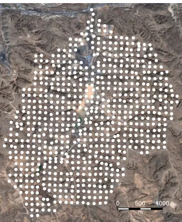
The data reports measurements made at 689 locations in the Liudaogou watershed, within the Loess Plateau, located 14 km west of Shenmu County, Shaanxi Province, China. Wang et al [38] provide a full description but in brief, this is a small watershed with an altitudinal range of 1081m to 1274m, a semi-arid climate with mainly grassland land use. The data were collected at locations on an approximate 100m by 100m grid (Figure 1) and analyzed in the laboratory to provide measurements of covariates commonly associated with STN and STP: soil organic carbon (SOCgkg), clay (ClayPC), silt (SiltPC), sand (SandPC), nitrate nitrogen (NO3Ngkg) and ammonium (NH4Ngkg). Some of the variables were transformed using natural logs (STN, SOCgkg, NO3Ngkg, NH4Ngkg) and square roots (STP, ClayPC), as was done by [38].
2.2
Linear regression and GWR
A standard linear regression for spatial data is specified as follows:
yi=β0+
m
X
j=1
βjxij+i (1)
where for observations indexed byi= 1, ...n,yiis the response variable,xijis the value
of thejthpredictor variable,mis the number of predictor variables,β
0is the intercept term, βjis the regression coefficient for thejthpredictor variable andiis the random error term.
GWR is similar in form to linear regression, except that GWR calculates a series of local linear regressions rather than one global one. A GWR model has locations associated with the coefficient terms:
JOSIS, Number N (YYYY), pp. xx–yy
Paper under review
4 AUTHOR1, AUTHOR2
0 500 1000 m
Figure 1: The sample locations and some context from the OpenStreetMap Bing layer
yi=β0(ui, vi) + m
X
j=1
βj(ui, vi)xij+i (2)
where(ui, vi)is the spatial location of theithobservation andβj(ui, vi)is a realization
of the continuous functionβj(u, v)at pointi. The geographical weighting results in data
nearer to the kernel center making a greater contribution to the estimation of local regres-sion coefficients at each local regresregres-sion calibration pointk. For this study, the weights were generated using abisquarekernel, which for the bandwidth parameter is defined by:
wik= (1−(dik/rk)2)2ifdik≤rk,wik= 0otherwise (3)
where the bandwidth can be specified as a fixed (constant) distance value, or in an adaptive, varying distance way, where the number of nearest neighbors is fixed (constant). In this case, fixed, distance-based kernel bandwidths were determined using the AIC-based model fit procedure. Fixed bandwidths were chosen to provide direct understand-ings of the spatial scales of relationship non-stationarity and because the data locations are regularly spaced.
2.3
Hyper-local GWR
In a hyper-local GWR, both the bandwidth and the regression model selection are opti-mized locally rather than globally across all local models as in a standard GWR. A sequence of bandwidths was investigated (from 200 m to 3700 m in steps of 50 m,n= 63) and at each location regression models of STN and STP were constructed using weighted data falling under the kernel. Then a stepwise AIC model selection procedure was applied. Thus for each location, 63 local regression models of STN and STP were constructed, for which 63
www.josis.org
Paper under review
HYPER-LOCALGWR 5
AIC scores were calculated. The ’best’ model and bandwidth combination at each location was that with the lowest AIC.
3
Results
3.1
Linear Regression
Linear regression models of STN and for STP were constructed from the six covariates and a stepwise AIC model selection procedure was applied. Tables 1 and 2 summarize the coefficient estimates and the selected covariates.
Full Selected
Estimate Std. Error t value Pr(>|t|) Estimate Std. Error t value Pr(>|t|)
(Intercept) -3.823 1.134 -3.371 0.001 0.011 0.035 0.314 0.754
SOCgkg 0.688 0.040 17.291 0.000 0.050 0.007 6.762 0.000
ClayPC 0.081 0.084 0.960 0.337 . . . .
SiltPC 0.028 0.010 2.912 0.004 0.004 0.001 4.678 0.000
SandPC 0.016 0.011 1.442 0.150 . . . .
NO3Ngkg 0.125 0.029 4.251 0.000 0.002 0.001 1.936 0.053
NH4Ngkg -0.138 0.074 -1.877 0.061 . . . .
R2:0.610 adjR2:0.607, AIC:1123.7 R2:0.141 adjR2:0.137 AIC:586.1
Table 1: Summary of the coefficient estimates arising from the Full and AIC selected linear regression models of STN.
Full Selected
Estimate Std. Error t value Pr(>|t|) Estimate Std. Error t value Pr(>|t|)
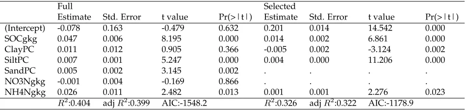
(Intercept) -0.078 0.163 -0.479 0.632 0.201 0.014 14.542 0.000
SOCgkg 0.047 0.006 8.195 0.000 0.014 0.002 6.861 0.000
ClayPC 0.011 0.012 0.905 0.366 -0.005 0.002 -3.124 0.002
SiltPC 0.007 0.001 5.247 0.000 0.004 0.000 11.206 0.000
SandPC 0.005 0.002 3.145 0.002 . . . .
NO3Ngkg -0.001 0.004 -0.169 0.866 . . . .
NH4Ngkg 0.026 0.011 2.482 0.013 0.001 0.001 2.276 0.023
R2:0.404 adjR2:0.399 AIC:-1548.2 R2:0.326 adjR2:0.322 AIC:-1178.9
Table 2: Summary of the coefficient estimates arising from the Full and AIC selected linear regression models of STP.
In the case of STN, the full model is being driven by SOCgkg along with SiltPC and NO3Ngkg are significantly associated with STN and model is similar to that described in Wang et al (2009) with an of 0.61 and all of the covariates positively associated with STN except NH4Ngkg. The AIC selected model did not include the ClayPC, SandPC and NH4Ngkg covariates. Observe that NO3Ngkg is not significantly associated with STN in the AIC selected model (at the 95% level). The significant predictors of STP in the full model were SOCgkg, SiltPC, SandPC and NH4Ngkg with an value of 0.40, again similar to the findings of Wang et al (2009). The selected model did not include the covariates for
JOSIS, Number N (YYYY), pp. xx–yy
Paper under review
6 AUTHOR1, AUTHOR2
NO3Ngkg and SandPC, but all retained covariates were significant. In both cases the se-lected models reflect the impact of silt and soil organic carbon in increasing the soil surface area supporting higher absorption capacities, and thus concentrations of STN and STP, as noted by Wang et al (2009). The AIC selected models are more parsimonious model but with weakerR2and adjustedR2values as would be expected.
Note that the selected model does not necessarily include covariates that are signif-icantly different from zero (via their t-values) and that covariate with non-significant t-values in the full model may be included in the selected model and may become significant (e.g. the ClayPC covariate for the STP regression). The key point is that the variance in STN and STP can be explained by two competing, but equally valid linear regression models. This concept is repeated locally in the subsequent GWR analyses and is a cornerstone of this paper.
3.2
Standard GWR
Linear regression models assume that the contributions to the model made by the differ-ent covariates are the same across the study area. In reality, this assumption of process spatial invariance may be violated. GWR seeks to quantify the spatial variation in the data relationships. In a standard GWR analysis, covariate selection is typically undertaken globally and the same regression model is constructed locally using local weighted data subsets. The local coefficient estimates are commonly mapped and local covariate selection (and goodness of fit evaluations) can be done by identifying local covariate t-values that indicate coefficients to be significantly different from zero (e.g. Harris et al. 2010b).
The optimal bandwidths for GWR models of STN and STP were found at 1026m and 1629m, respectively. These were used to calibrate the GWRs constructed at each of the sample locations in Figure 1. The local coefficient estimates from these are summarized in Tables 3 and 4. The GWR coefficients for STN show considerable spatial variation (via the inter-quartile range, IQR) and much less is found in the local STP models, as also reflected in its larger bandwidth. For example, in the STN GWR model the coefficient estimates for SandPC and NO3Ngkg have IQRs of 0.0156 and 0.1247, respectively, while in the STP GWR model these have relatively small IQRs (0.0023 and 0.0077, respectively).
Min. 1st Qu. Median Mean 3rd Qu. Max. IQR Global Intercept -11.8600 -4.9410 -2.8260 -3.0400 -0.8880 2.0820 4.0530 -3.8229 SOCgkg 0.4050 0.6137 0.6730 0.6760 0.7509 0.9294 0.1372 0.6882 ClayPC -0.3965 -0.0162 0.0865 0.0752 0.1630 0.5661 0.1792 0.0811 SiltPC -0.0295 0.0012 0.0166 0.0201 0.0390 0.0898 0.0378 0.0284 SandPC -0.0414 -0.0092 0.0068 0.0099 0.0316 0.0917 0.0408 0.0156 NO3Ngkg -0.1191 0.0399 0.0909 0.1282 0.1666 0.6079 0.1267 0.1247 NH4Ngkg -0.8360 -0.2313 -0.1115 -0.1661 -0.0395 0.1237 0.1918 -0.1384
Table 3: The distributions of the coefficient estimates arising from a GWR model of STN.
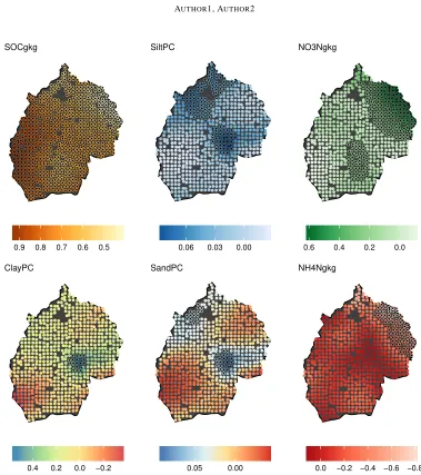
The spatial variations in the coefficient estimates arising from the two GWR models are mapped in Figures 2 and 3 and indicate the relative importance of the contribution made to each local model by each covariate at each location. They confirm that there is much greater spatial variation in the relationships associated with STN than with STP.
www.josis.org
Paper under review
HYPER-LOCALGWR 7
Min. 1st Qu. Median Mean 3rd Qu. Max. IQR Global Intercept -0.7236 -0.2119 -0.1046 -0.0683 0.0640 0.6685 0.2759 -0.0781 SOCgkg 0.0183 0.0371 0.0410 0.0422 0.0487 0.0599 0.0116 0.0469 ClayPC -0.0673 -0.0130 0.0132 0.0063 0.0261 0.0598 0.0391 0.0110 SiltPC 0.0024 0.0059 0.0081 0.0078 0.0098 0.0119 0.0039 0.0074 SandPC 0.0029 0.0038 0.0050 0.0051 0.0061 0.0104 0.0023 0.0049 NO3Ngkg -0.0096 -0.0016 0.0027 0.0031 0.0061 0.0434 0.0077 -0.0007 NH4Ngkg -0.1505 0.0000 0.0186 0.0180 0.0412 0.0722 0.0412 0.0263
Table 4: The distributions of the coefficient estimates arising from a GWR model of STP.
The t-values in Figures 2 and 3 provide an indication of where local coefficients are sig-nificant and thus where a covariate is an important predictor of STN or STP. This provides an indication of local covariate selection from the full model and is analogous to the global full models reported in Tables 1 and 2. For example, it is evident in both GWR models that SOCgkg is strongly and significantly associated with STN and STP across all locations, but the strength of this association varies spatially. Whereas significant coefficient estimates of NO3Ngkg are highly localized in each GWR model indicting strong associations in the north east and center of the study area with STN and strong associations in the north with STP. In general, significant relationships are much more localized for STN than for STP.
3.3
Hyper-local GWR
The GWR analysis applied the same kernel bandwidth and included the same full set of covariates in each local regression model. Figures 2 and 3 display the spatial distribution of the GWR coefficient estimates and a degree of local model selection is possible through exploration of the local t-values associated with the local coefficient estimates. This is a standard application of GWR, supporting investigations of process heterogeneity with re-spect to spatially-varying relationships.
The hyper-local GWR approach provides an alternative interpretation of localized re-gression through local model selection and local bandwidth optimization. It builds on pre-vious GWR studies that have identified analytical advantages when locally-determined, non-constant bandwidths are applied [33, 34] and when covariate selection is determined locally (e.g. [41]). It combines these localized characteristics but the ultimate objective is entirely different to the studies of Paez and Wheeler: Paez et al [33, 34]. were concerned about modeling a non-stationary error variance in GWR via a parametric approach and Wheeler [41] sought to address local collinearity in GWR via a lasso approach.
For each of the 689 data points, the hyper-local GWR identified the components of the best fitting model for each of the 63 bandwidths (from 200 m to 3700 m in intervals of 50 m) and the associated AIC score. Thus it was possible to determine the best fitting model, with the lowest AIC score at each location.
3.3.1 Local bandwidth selection
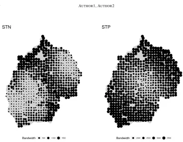
Figure 4 shows bandwidths with the lowest AIC scores from the hyper-local GWR mod-els of STN and STP. They exhibit different spatial patterns and characteristics. The STN bandwidths range from 200-1800 m, with larger bandwidths (say, 1000-1800 m) traversing
JOSIS, Number N (YYYY), pp. xx–yy
Paper under review
8 AUTHOR1, AUTHOR2
0.5 0.6 0.7 0.8 0.9 SOCgkg
−0.2 0.0 0.2 0.4 ClayPC
0.00 0.03 0.06 SiltPC
0.00 0.05
SandPC
0.0 0.2 0.4 0.6 NO3Ngkg
−0.8 −0.6 −0.4 −0.2 0.0 NH4Ngkg
Figure 2: Spatial variation in coefficient estimates from a standard GWR model of STN. Significant t-values are indicated by the black shaded points.
from the south-east to the north-west. This suggest that local regressions in this area band are informed by data subsets of a similar size to that found with standard GWR (with its constant bandwidth of 1026 m). Elsewhere, the bandwidths are much smaller (200-1000 m), so that local regressions in these areas are informed by much smaller data subsets. The distribution of bandwidths in the hyper-local GWR model, is on the whole indicative of increased localized spatial heterogeneity in data relationships, which is more than that suggested by the standard GWR analyses, above.
Conversely, the STP bandwidths range from 1500 -3700 m and are much larger almost everywhere than the constant bandwidth for standard GWR at 1629 m. Thus, most local
www.josis.org
Paper under review
HYPER-LOCALGWR 9
0.5 0.6 0.7 0.8 0.9 SOCgkg
−0.2 0.0 0.2 0.4 ClayPC
0.00 0.03 0.06 SiltPC
0.00 0.05
SandPC
0.0 0.2 0.4 0.6 NO3Ngkg
−0.8 −0.6 −0.4 −0.2 0.0 NH4Ngkg
Figure 3: Spatial variation in coefficient estimates from a standard GWR model of STP. Significant t-values are indicated by the black shaded points.
regressions of hyper-local GWR are informed by much larger data subsets. Only to the center of the study area are bandwidths from hyper-local GWR of similar size to a standard GWR. The larger bandwidths indicate reduced spatial heterogeneity to that found with standard GWR, and suggests spatial homogeneity in the relationships (i.e. tending to the global regression).
JOSIS, Number N (YYYY), pp. xx–yy
Paper under review
10 AUTHOR1, AUTHOR2
Bandwidth 500 1000 1500
STN
Bandwidth 2000 2500 3000 3500
STP
Figure 4: Spatial variation in local bandwidth size (in metres) of the hyper-local GWR mod-els of STN and STP.
3.4
Local covariate selection and distribution of coefficient t-values
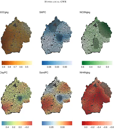
Investigating the spatial variation in bandwidth size is only one aspect of hyper-local GWR and should be coupled with consideration of local covariate selection. Table 5 summarizes how many times each covariate was selected using stepwise AIC at each of the 689 loca-tions in the hyper-local GWR models. There are a number of interesting points. STN model selection for the global regression (Table 1 excluded ClayPC, SandPC and NH4Ngkg, while these are now selected in 522, 641 and 439 out of 689 hyper-local models, respectively. STP model selection for the global regression (Table 2) excluded SandPC and NO3Ngkg, while these are now selected in 689 and 170 out of 689 local models, respectively. Additionally, three covariates were always selected regression (SOCgkg, SiltPC and SandPC), whereas for STN none were. This suggests that there are potentially interesting local interactions between covariates which are missed in standard GWR in which all six covariates are in-cluded in the model for all 689 local regressions.
Figures 5 and 6 indicate where different covariates were selected for inclusion in the local regression models under the hyper-local GWR and where the associated coefficient estimates were found to be locally significant via their t-values. When these are compared with maps of t-values in Figures 2 and 3 for standard GWR, some large local differences are evident, especially for the STN process.
For example, in the STN processes (comparing Figures 2 and 5), SandPC is a significant covariate in most locations in hyper-local GWR model. In the standard GWR model (Figure 2 it only significant in two sub-regions to the north and center of the study area. Whilst,
www.josis.org
Paper under review
HYPER-LOCALGWR 11
STN STP SOCgkg 657 689 ClayPC 522 527 SiltPC 505 689 SandPC 641 689 NO3Ngkg 476 170 NH4Ngkg 439 425
Table 5: Number of sample locations where different covariates were selected in hyper-local GWR.
NH4Ngkg in the standard GWR model of STN is significant in the north-west of the study area, but has a much wider significance in the hyper-local GWR model. These results in-dicate that when the bandwidth and covariate selection tends to be more localized under the hyper-local GWR, then significant non-stationary relationships result, that are not ap-parent with standard GWR. Similar interpretations of these findings for STN relationships with SiltPC, NO3Ngkg and ClayPC while it appears that STNâ ˘A ´Zs relationship to SOCgkg is consistent across both GWR forms. Note also that hyper-local GWR tends to provide spatially-disjoint areas of covariate selection and coefficient significance, reflecting highly localized processes. For the STP process, comparing Figures 3 and 6, there are very sim-ilar patterns for significant coefficients from hyper-local GWR and from a standard GWR for all six covariates, although NO3Ngkg, SandPC, ClayPC and NH4Ngkg show enlarged localized areas of significance under the hyper-local model. Note that NO3Ngkg is only selected in 170 sample locations in hyper-local GWR (see Table 5) and these center in the north, precisely where standard GWR shows the NO3Ngkg relationships as significant.
Clearly, these results indicate that when the bandwidth and covariate selection tend towards the global solution, as with the hyper-local GWR of STP the non-stationary rela-tionships that result from a hyper-local GWR are broadly similar for both forms of GWR. However, where localized spatial heterogeneity is present in data relationships, as with STN, the hyper-local GWR provides a more spatial nuanced indication of the localization than a standard GWR analysis.
3.5
Comparisons of global and local model fit
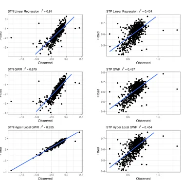
The final analysis compared the three different regression models in the degree to which they (in-sample) predict STN and STP. The scatterplots in Figure 7 show fitted values against observed values for these six models. For STN, the model fits improve with increas-ing spatial nuance, from linear regression (full model), to standard GWR and to hyper-local GWR (R2 of 0.61, 0.68 and 0.94, respectively). Rather surprisingly, there is little improve-ment in model fit from the linear regression to standard GWR. The strong predictive per-formance of hyper-local GWR can be attributed to the local tightening of bandwidths and variable selection. For STP, the model fits do not improve in the same way. There is a moderate increase from linear regression (full model) to standard GWR but then a small decrease to the hyper-local GWR (R2of 0.40, 0.47 and 0.45 respectively). The decrease in R2observed for hyper-local GWR simply reflects that this model is actually not as local as standard GWR, as the bandwidths for hyper-local GWR tend to be larger and the process tends towards the global fit.
JOSIS, Number N (YYYY), pp. xx–yy
Paper under review
12 AUTHOR1, AUTHOR2
SOCgkg
ClayPC
SiltPC
SandPC
NO3Ngkg
NH4Ngkg
Figure 5: The spatial distribution of the selected covariates included in each hyper-local GWR model of STN, with those with significant t-values are indicated by a larger symbol.
Care must be taken in the interpretation of model fit results, as any form of localised regression will tend to provide an improved prediction accuracy, the more complex it gets (hence the strong performance of local GWR for STN). Furthermore, although hyper-local GWR is shown to improve fit for the STN process, this has little predictive value, as hyper-local GWR cannot be used as an of-sample predictor. This is because the out-of-sample prediction does not have its own local bandwidth, whereas for standard GWR, the global bandwidth can be used [22]. Thus, hyper-local GWR is solely for guiding spatial exploration and inference only, as demonstrated in this study.
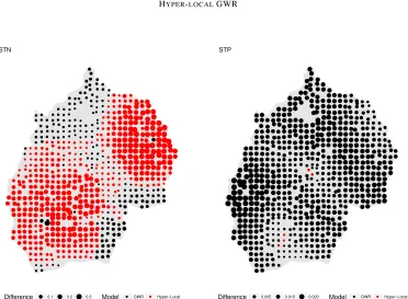
It is important to investigate local model fit characteristics so that the outputs in Figures 2 to 6 can be placed in better context and geographically contrasted. Figure 8 compares the localR2 values for standard GWR and hyper-local GWR models for STN and STP and indicates that hyper-local GWR provides a better fit in 503/689 and 5/689 locations for STN and STP, respectively. Thus, for the STN process, the local regressions of standard GWR could be considered sub-optimal in 73% of the locations, whilst for the STP process,
www.josis.org
Paper under review
HYPER-LOCALGWR 13
SOCgkg
ClayPC
SiltPC
SandPC
NO3Ngkg
NH4Ngkg
Figure 6: The spatial distribution of the selected covariates included in each hyper-local GWR model of STP, with those with significant t-values are indicated by a larger symbol.
the local regressions of standard GWR are in general, reasonable. The magnitude of the differences are much greater for STN than for STP. If Figure 8 is compared with Figure 4, the areas where a hyper-local approach provides a better model fit for STN directly corre-spond to those where a much smaller local bandwidth was selected. This behavior is not so apparent for the STP process.
The maps in Figure 8 confirm what has already been described. For STN, hyper-local GWR suggests a more localized relationship process where local model fit can improve using fewer data points and fewer covariates. Standard GWR is under-fitting the true non-stationary relationship process and this effect is not uncommon (e.g. [24]). Conversely, it is always possible that hyper-local GWR is over-fitting. The STN process is in general, well-informed by the six covariates. For STP, hyper-local GWR suggests more moderately spatially-varying relationships but where local model fits are similar (slightly weaker) to that found for standard GWR. Thus, the application of hyper-local GWR provides little
JOSIS, Number N (YYYY), pp. xx–yy
Paper under review
14 AUTHOR1, AUTHOR2
−3 −2 −1 0
−7.5 −5.0 −2.5 0.0 2.5
Observed
Fitted
STN Linear Regression r2 = 0.61
−4 −3 −2 −1 0
−7.5 −5.0 −2.5 0.0 2.5
Observed
Fitted
STN GWR r2 = 0.679
−9 −6 −3 0
−7.5 −5.0 −2.5 0.0 2.5
Observed
Fitted
STN Hyper Local GWR r2 = 0.935
0.5 0.6 0.7
0.5 1.0
Observed
Fitted
STP Linear Regression r2=0.404
0.4 0.5 0.6 0.7 0.8
0.5 1.0
Observed
Fitted
STP GWR r2=0.467
0.4 0.5 0.6 0.7
0.5 1.0
Observed
Fitted
STP Hyper Local GWR r2=0.454
Figure 7: Fitted values for STN and STP arising from linear regression, standard GWR and hyper local GWR models against observed values.
www.josis.org
Paper under review
HYPER-LOCALGWR 15
Difference 0.1 0.2 0.3 Model GWR Hyper−Local STN
Difference 0.005 0.010 0.020 Model GWR Hyper−Local STP
Figure 8: Maps of the difference in localR2values under standard GWR and hyper-local GWR models. Locations in red indicate where a hyper-local GWR model resulted in a better fitting model and (black for GWR) and the size of the plot characters indicate the magnitude of the difference.
value to an extended use of nearby data points with often fewer covariates for its local regressions. The STP process, is in general, not well-informed by the six covariates.
4
Discussion
GWR is an inherently exploratory approach for examining and investigating process non-stationarity in data relationships. The proposed hyper-local GWR extends these investi-gations further. It provides an alternative and complementary interpretation of localized regression by locally selecting the most parsimonious model (by local sample and covariate size), for which spatially distributed coefficient estimates and t-values can also be found. The local selection of the most parsimonious model is analogous to what is commonly done in a global analysis, where a summary of the full model is presented alongside a reduced, selected covariates model.
The investigations show that where the non-stationarity of relationships tend towards the global, as with STP, the results are similar to a standard GWR (compare Figures 3 and 6). However, where localized spatial heterogeneity and spatial non-stationarity are present, as with STN, the hyper-local GWR provides a more spatially nuanced indication of the localization than a standard GWR analysis (compare 2 and 5). Thus the hyper-local GWR results can be used to guide the direction of the next steps. Further analysis of the
JOSIS, Number N (YYYY), pp. xx–yy
Paper under review
16 AUTHOR1, AUTHOR2
STN could consider adopting a more sophisticated spatially-varying coefficient model (e.g. [18]), including models that accounts for non-linearity (e.g. [2]. Further analysis of STP could consider a spatially-autocorrelated regression given that its GWR analyses were not entirely promising (e.g. [24]).
Determining local bandwidth size and local covariate selection is also in the same spirit as (but with entirely different objectives to) the GWR models of Paez et al. [33, 34], Wheeler [41] and Yoneoka et al. [42], some of which are analogous to developments in lo-cal (attribute-space) regression [28, 37] from which GWR originates [7, 30]. The exploratory and enhanced spatial nuance of hyper-local GWR reflects recent developments within the broad family of GWR methods that has promoted wider consideration of scale. These in-clude hierarchical GWR models [25] and also flexible bandwidth GWR models [17, 27, 29] that select different bandwidths for each dependent/independent data relationship, rather than for each location as here. These multi-scale GWR models are closely aligned to the spatially-varying coefficient models of Gelfand et al [18] and Murakami et al [31].
There are a number of considerations relating to the GWR models applied and demon-strated in this study. The first is collinearity. Standard GWR and hyper-local GWR are not designed to address collinearity issues, but here hyper-local GWR could be adapted to mit-igate against such issues, in a similar manner to that proposed for standard GWR (e.g. [2, 6, 39]). The second concerns multiple hypothesis tests (MHTs), where GWRt-values were presented in an uncorrected form that inherently leads to the false discovery rate problem. Here the MHT corrections suggested by da Silva and Fotheringham [13] could be adopted for both standard and hyper-local GWR t-value outputs. A third consideration is the choice of kernel, the bandwidth type (fixed by distance, as used here, or fixed by sample size) and the choice of distance metric, all of which effect perspectives of coefficient non-stationarity, where it would be interesting to examine the degree of difference between the STN and STP standard and hyper-local GWR models under such different parameterization choices. Gollini et al. [19] provides overviews of these considerations. A fourth and more salient consideration for the research described in this paper is the use of AIC scores to select both local bandwidths and local regression models. AIC [1, 26] seeks to optimise model parsimony by trading off prediction accuracy and complexity. Other measures of fit could be applied including some kind of cross-validation measure of residual errors. There have been a number of arguments made in the context of information theory about the choice of model selection method and their associated measures of fit. Future work will investigate CV approaches as they would be expected result in different local model selection. In terms of information criteria, alternatives to AIC exist such as Bayesian Information Criterion (BIC) and Deviance Information Criterion (DIC) [35]. The key in determining which model selection method to use is to understand the logics of each approach and how they relate to the study objectives and even the underlying objectives of data collection. For example, AIC and BIC provide different approaches for model comparison [8]. BIC seeks to deter-mine the â ˘AŸtrueâ ˘A ´Z model and, if any particular candidate model represents the genuine data-generating mechanism, BIC will select such a model. It is said to be asymptotically consistent because it seeks to select the true model. By contrast AIC seeks to pragmatically select a model by trading-off explanations of the data with prediction strength. Despite these theoretical differences Spiegelhalter et al [36] note that â ˘AŸit is perhaps therefore rather surprising how often these two criteria produce similar rankings of candidate mod-elsâ ˘A ´Z (p. 486) with the only real differences found in the size of the penalty scores [14]. Future work for both hyper-local and standard GWR will investigate the use of different
www.josis.org
Paper under review
HYPER-LOCALGWR 17
model selection criteria, the logics associated with the local models being constructed and under-lying process spatial heterogeneity.
5
Conclusions
Local statistical approaches such as GWR are inherently exploratory in nature. They seek to confirm or refute spatial heterogeneity in spatial data structure, processes and statistical relationships. The hyper-local GWR approach described in this paper provides a useful counter view of local regression modeling to that found with standard GWR. Standard GWR applies the same regression model at each location and uniformly sets the same kernel bandwidth everywhere. The hyper-local GWR approach evaluates different ker-nel bandwidths at each location and selects the most parsimonious local regression. Where spatial non-stationarity exists, the hyper-local GWR provides a more spatially nuanced in-dication of the localization than a standard GWR analysis and can be used to suggest the di-rection of further analyses and investigations. Undertaking a hyper-local GWR alongside a GWR allows coefficient estimates,t-values and bandwidths to be compared for differences and similarities. Specifically, a dual GWR approach that examines the spatial distribution of local covariate selection and the local bandwidth size supports a deeper understanding of the local and scale-related characteristics of the spatial process under investigation.
Acknowledgments
This work was supported by National Natural Science Foundation of China (NSFC) and the Natural Environment Research Council (NERC) Newton Fund through the China-UK collaborative research on critical zone science (No. 41571130083 and NE/N007433/1), the NSFC (No.41530854) and UK Biotechnology and Biological Sciences Research Council grant (BBSRC BB/J004308/1). All of the analyses and mapping were undertaken in R 3.3.2 the open source statistical software. The GWR analyses used the GWmodel package, v2.0-1 (Gollini et al, 2015). The data and code will be available to interested researchers on request. AC conceived, and led the design and implement ion of the analysis; YW collected and processed the data used in the analysis; PH guided the analysis. All authors contributed to interpreting the results, refining the analysis and the writing of the manuscript.
6
References
I will learn bibtex by the time this gets reviewed and will format all references appropri-ately.
[1] Akaike, H. 1973. Information Theory and an Extension of the Maximum Likeli-hood Principle. In BN Petrov, F Csaki (eds.), 2nd Symposium on Information Theory, pp. 267â ˘A¸S281. Akademiai Kiado, Budapest.
[2] BÃ ˛arcena, M. J., MenÃl’ndez, P., Palacios, M. B., and Tusell, F. 2014. Alleviating the effect of collinearity in geographically weighted regression. Journal of Geographical Systems, 16(4), 441-466.
JOSIS, Number N (YYYY), pp. xx–yy
Paper under review
18 AUTHOR1, AUTHOR2
[3] Basile, R., M. Durban, R. Minguez, J.M. Montero, and J. Mur (2014). Modeling re-gional economic dynamics: Spatial dependence, spatial heterogeneity and non-linearities. Journal of Economic Dynamics and Control 48, 229-245.
[4] Brunsdon, C., Fotheringham, A.S. and Charlton, M., 2002. Geographically weighted summary statisticsâ ˘AˇTa framework for localised exploratory data analysis.Computers, En-vironment and Urban Systems,26(6), pp.501-524.
[5] Brunsdon, C., Fotheringham, S. and Charlton, M., 2007. Geographically weighted discriminant analysis.Geographical Analysis,39(4), pp.376-396.
[6] Brunsdon, C., Charlton, M. and Harris, P. 2012. Living with Collinearity in Local Re-gression Models. In Proceedings of the 10th International Symposium on Spatial Accuracy Assessment in Natural Resources and Environmental Sciences. Brasil.
[7] Brunsdon, C.F., Fotheringham, A.S. and Charlton M. (1996). Geographically Weighted Regression - A Method for Exploring Spatial Non-Stationarity, Geographic Anal-ysis, 28: 281-298.
[8] Burnham KP and Anderson DR (2004) Multimodel inference: Understanding AIC and BIC in model selection. Sociological Methods and Research 33(2): 261â ˘A¸S304.
[9] Chiles, J.P. and Delfiner, P., 2009.Geostatistics: modeling spatial uncertainty. John Wiley and Sons.
[10] Comber, A., Li, T., LÃij, Y., Fu, B. and Harris, P. (2017a) Geographically Weighted Structural Equation Models: spatial variation in the drivers of environmental restoration effectiveness. In Societal Geo-Innovation, 20th AGILE conference proceed-ings, available from https://agile-online.org/images/conference 2017/Proceedings2017/ shortpapers/94 ShortPaper in PDF.pdf
[11] Comber A, Brunsdon CF, Charlton M and Harris P (2017b). Geographically weighted correspondence matrices for local change analyses and error reporting: mapping the spatial distribution of errors and change. Remote Sensing Letters, 8(3): 234-243
[12] Comber A.J., (2013). Geographically weighted methods for estimating local sur-faces of overall, user and producer accuracies. Remote Sensing Letters, 4(4): 373-380
[13] da Silva, A.R. and Fotheringham, A.S., 2016. The multiple testing issue in geo-graphically weighted regression.Geographical Analysis,48(3), pp.233-247.
[14] Dziak, J.J., Coffman, D.L., Lanza, S.T. and Li, R., 2012. Sensitivity and specificity of information criteria.The Methodology Center and Department of Statis-tics, Penn State, The Pennsylvania State University,16(30), p.140 available from https://methodology.psu.edu/media/techreports/12-119.pdf
[15] Foody, G. M. (2005). Local characterization of thematic classification accuracy through spatially constrained confusion matrices. International Journal of Remote Sensing, 26, 1217â ˘A¸S1228.
[16] Fotheringham, A. S., C. Brunsdon, and M. Charlton. (2002). Geographically Weighted Regression: The Analysis of Spatially Varying Relationships. Chichester: Wiley
[17] Fotheringham, A.S., Yang, W., and Kang, W. (2017) Multiscale Geographically Weighted Regression (MGWR). Annals of the American Association of Geographers DOI: 10.1080/24694452.2017.1352480
[18] Gelfand, A.E., Kim, H.J., Sirmans, C.F. and Banerjee, S., 2003. Spatial modeling with spatially varying coefficient processes.Journal of the American Statistical Associa-tion,98(462), pp.387-396.
www.josis.org
Paper under review
HYPER-LOCALGWR 19
[19] Gollini I, Lu B, Charlton M, Brunsdon C and Harris P (2015). GWmodel: an R Pack-age for exploring Spatial Heterogeneity using Geographically Weighted Models. Journal of Statistical Software 63 (17), 1-50
[20] Harris, P., Charlton, M. and Fotheringham, A.S., 2010a. Moving window kriging with geographically weighted variograms.Stochastic Environmental Research and Risk As-sessment,24(8), pp.1193-1209.
[21] Harris P, Fotheringham AS, Juggins S (2010b) Robust geographically weighed re-gression: a technique for quantifying spatial relationships between freshwater acidification critical loads and catchment attributes. Annals of the Association of American Geographers 100(2): 286-306
[22] Harris P, Fotheringham AS, Crespo R, Charlton M (2010c) The use of geographically weighted regression for spatial prediction: an evaluation of models using simulated data sets. Mathematical Geosciences 42:657-680
[23] Harris, P., Brunsdon, C., Charlton, M., 2011. Geographically weighted princi-pal components analysis. International Journal of Geographical Information Science 25, 1717â ˘A¸S1736.
[24] Harris P, Brunsdon C, Lu B, Nakaya T, Charlton M (2017) Introducing bootstrap methods to investigate coefficient non-stationarity in spatial regression models. Spatial Statistics 21: 241-261
[25] Harris R, G Dong, Zhang W (2013) Using Contextualized Geographically Weighted Regression to Model the Spatial Heterogeneity of Land Prices in Beijing, China. Transac-tions in GIS 17(6):901-919
[26] Hurvich CM, Simonoff JS, Tsai CL (1998). Smoothing Parameter Selection in Nonpara- metric Regression Using an Improved Akaike Information Criterion. Journal of the Royal Statistical Society B, 60(2), 271â ˘A¸S293.
[27] Leong, Y. Y., and Yue, J. C. (2017). A modification to geographically weighted re-gression. International Journal of Health Geographics, 16 (1), 11.
[28] Loader, C. (2004). Smoothing: Local Regression Techniques. Handbook of Compu-tational Statistics. J. Gentle, W. Hardle and Y. Mori. Heidelberg, Springer-Verlag.
[29] Lu, B., Brunsdon, C., Charlton, M. and Harris, P., 2017. Geographically weighted regression with parameter-specific distance metrics.International Journal of Geographical Information Science,31(5), pp.982-998.
[30] McMillen DP, McDonald JF (1997) A nonparametric analysis of employment den-sity in a polycentric city. Journal of Regional Science 37(4):591-612 [31] Murakami, D., Yoshida, T., Seya, H., Griffith, D.A., and Yamagata, Y. (2017) A Moran coefficient-based mixed effects approach to investigate spatially varying relationships. Spatial Statistics, 19, 68-89.
[32] Openshaw, S., 1996. Developing GIS-relevant zone-based spatial analysis meth-ods.Spatial analysis: modelling in a GIS environment, pp.55-73.
[33] Paez, A., T. Uchida, et al. (2002a). A general framework for estimation and inference of geographically weighted regression models: 1. Location-specific kernel bandwidths and a test for locational heterogeneity. Environment and Planning A 34: 733-754.
[34] Paez, A., T. Uchida, et al. (2002b). A general framework for estimation and in-ference of geographically weighted regression models: 2. Spatial association and model specification tests. Environment and Planning A 34: 833-904.
JOSIS, Number N (YYYY), pp. xx–yy
Paper under review
20 AUTHOR1, AUTHOR2
[35] Spiegelhalter, D.J., Best, N.G., Carlin, B.P. and Van Der Linde, A., 2002. Bayesian measures of model complexity and fit.Journal of the Royal Statistical Society: Series B (Sta-tistical Methodology),64(4), pp.583-639.
[36] Spiegelhalter, D.J., Best, N.G., Carlin, B.P. and Linde, A., 2014. The deviance infor-mation criterion: 12 years on.Journal of the Royal Statistical Society: Series B (Statistical Methodology),76(3), pp.485-493.
[37] Vidaurre, D., Bielza, C. and Larraôsaga, P., 2012. Lazy lasso for local regression. Computational Statistics, pp.1-20.
[38] Wang, Y., Zhang, X. and Huang, C., 2009. Spatial variability of soil total nitrogen and soil total phosphorus under different land uses in a small watershed on the Loess Plateau, China. Geoderma, 150(1), pp.141-149.
[39] Wheeler, D. 2007. Diagnostic Tools and a Remedial Method for Collinearity in Geographically Weighted Regression. Environment and Planning A, 39(10), 2464â ˘A¸S2481.
[40] Wheeler, D. and Tiefelsdorf, M. 2005. Multicollinearity and Correlation among Regression Co-efficients in Geographically Weighted Regression. Journal of Geographical Systems, 7(2), 161â ˘A¸S187.
[41] Wheeler, D.C., 2009. Simultaneous coefficient penalization and model selection in geographically weighted regression: the geographically weighted lasso. Environment and planning A, 41(3), pp.722-742.
[42] Yoneoka, D., Saito, E. and Nakaoka, S., 2016. New algorithm for constructing area-based index with geographical heterogeneities and variable selection: An application to gastric cancer screening. Scientific Reports, 6: 26582.
www.josis.org