On-Board Correction of Systematic Odometry Errors
in Differential Robots
S. Maldonado-Bascón1,† , R. J. López-Sastre1,†, F.J. Acevedo-Rodríguez1,†and P. Gil-Jiménez1,† 1 Dpto. de Teoría de la Señal y Comunicaciones
Escuela Politecnica Superior Universidad de Alcalá Alcalá de Henares (Madrid)
http://agamenon.tsc.uah.es/Investigacion/gram
* Correspondence: e-mail: [email protected] Version November 8, 2018 submitted to Preprints
Abstract: An easier method for the calibration of differential drive robots is presented. Most of the
1
calibration is done on-board and it is not necessary to expend too much time taking note of the robot’s
2
position. The calibration method does not need a big free space to perform the tests. The bigger space
3
is just in a straight line, which is easy to find. Results with the proposed method are compared with
4
those from UMB as a reference, and they show very little deviation while the proposed calibration is
5
much simpler.
6
Keywords:differential drive robot; calibration; systematic error.
7
1. Introduction 8
Odometry based on encoder information is the way used to get the relative position on most of
9
the differential drive robots. In this paper, we describe our solution for the calibration of such robots in
10
order to avoid systematic error.
11
1.1. Odometry calculations 12
As a summary, we include the odometry expresions for differential robots, in order to point out
13
the dependency of those calculations on the parameters we need to calibrate. Iteratively, the position
14
of the robot is obtained by approximation. For a given iteration,PRandPLrepresents the pulses of the 15
right and left encoder respectively.
16
The factor that converts the pulses into mm of linear displacement isCm, given by
Cm= πD Ce
whereDis the wheel diameter andCeis the number of pulses per revolution of our encoder. So, in each iterationi, the distance travelled by the right and left wheels∆UR/L,iis
∆UR/L,i=CmPR/L,i
The distance travelled by the centre of the wheel axis and the change in the orientation in each iteration are given by
∆Ui = 1
2(∆UR,i+∆UL,i) ∆θi =
1
b(∆UR,i−∆UL,i)
wherebis the wheelbase: the distance from the contact point of both wheels with the floor. The global orientation is
θi =θi−1+∆θi
Yi =Yi−1+∆Uisin(θi)
As can be seen from these equations, they depend onDandb, whereDwill beDRandDLbecause of 17
the two wheels.
18
1.2. Related work 19
Deviations in these parameters produce systematic errors, and a calibration process is necessary
20
for differential drive robots due to construction errors. Non-systematic errors will appear due to a
21
slippery or unregular floor, but these are not our objective in this paper.
22
[1] and [2] are the main references for systematic odometry error correction. In [1] a 4 m side square
23
is travelled clockwise and counterclockwise in order to correct the relation of the wheel diameters and
24
the distance between the wheels.
25
There are 3 sources of error. First, in the average wheel diameterDavg, we consider a scaling factor Esfrom the nominal value.
Davg=EsDnom
Second, the fact that the wheel diameters are unequal. Depending on the construction of the wheel, this error can be larger or smaller. If we take the diameterDRof the right wheel as a reference, the left diameterDLis given by the factorEd:
DL =EdDR
The last error source to adjust is the wheelbase,b, so the relation between the actual wheelbase,bact and the nominal is
bact=Ebbnom
Some papers have proposed correctingEdandEb[1] and [3]. For example, in [4], the 3 parameters are 26
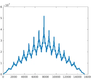
adjusted.
27
In [4], two experiments are proposed. A movement forward with a rotation ofπand then coming 28
back, one with a clockwise rotation and one counterclokwise. Simulation results are shown, but it
29
does not indicate the number of iterations of the experiments. In [1], travelling over a 4 m side square
30
both counterclockwise and clockwise is proposed, 5 times each. One of the problems is that you need
31
a freee space of 4 m×4 m plus the dimensions of the robot with a regular non-slippery floor. They
32
also assumedEs =1, so you need to calibrateDavgbefore starting the experiments. The robot must be 33
placed carefully in the same position and orientation for the 10 trials. In [5], the expresions from [1] are
34
corrected. They also analyse the effect of the square path size: 1 m×1 m was not successful, because
35
is was too small. Their expressions show in simulation better convergence if the experiment is iterated
36
and better results for 2 m×2 m. In [3] a bidirectional circular path test is proposed to estimate the
37
correction factors. They said: ‘the low noise procedure allows to obtain good results without the need
38
to repeat the experimets.’ They point out that a circular path of 5 m in diameter, that it is even worse
39
than the 4 m square recommended in [1].
40
A description of self-calibration is presented in [6]. It is based on a laser range finder that allows
41
high accuracy measurement. Similar papers using laser range finders can be found in the literature,
42
but those are not related with the present paper.
43
We are looking for a method for occasional calibration that will require little time. Calibration
44
is important to increase accuracy and to reduce the number of corrections needed using absolute
45
position estimation: these can be reduced if the relative position is accurate. In the present paper, a
46
calibration method to reduce systematic relative position error for a differential drive mobile robot
47
is presented. The proposed method needs just enough space for the robot to turn and to perform a
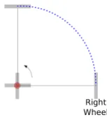
Figure 1.Robot scheme while turning with left wheel stopped.
3 m long straight movement. It is also important to note that most of the data for the calibration are
49
obtained and calculated on-board. It is not necessary to be careful with the initial position of the robot.
50
Both features allow calibrating the robot very quickly.
51
Our research group has been working on developing many different technical aids under the
52
solidarity program “Padrino Tecnológico”(http: //padrinotecnologico.org/), from walkers to electric
53
wheelchairs. This is an approach to use robots for assistive tasks. Orientation for people with cognitive
54
disorder is being stressed, and helping to increase their autonomy is the first goal of this project,
55
although many other functionalities can be included using the same hardware. This is the second
56
platform we have worked on. The previous one was too small to get into disabled attention centres.
57
2. Calibration method 58
2.1. Estimation of Ed 59
The proposed calibration method aims at reducing the time required to perform a calibration. We are searching for the actualDR,DLandb. The first experiment looks for the relationEd=DR/DL: the robot will describe a circular path with the left wheel stopped forNrounds. Then, this is repeated with the right wheel stopped for anotherNrounds. Fig.1represents the robot while turning with a stopped left wheel. The distance travelled,s, in each round, can be expressed in different ways depending on theeffectivewheelbase, and the number of pulses in each roundP1RandP1L:
s=2πb= P1RπDR ce
= P1LπDL
ce (1)
wherecepulses/rev is a constant to translate wheel turns to pulses. 60
Using Equation (1) yields
Ed= DL DR
= P1R
P1L
The movements involved in this test suffer from one problem: stopped wheels need low friction
61
to perform the circular movement of the robot but enough friction to get the wheel at the same point.
62
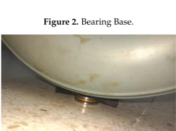
When the test is done on a slippery floor, a small piece (see Fig.2) has been designed to achieve this
63
goal, so now the wheel pivots on that piece over an axial bearing. Fig.3illustrate the situation of the
64
wheel during the test: the wheel, the piece, and the axial bearing are visible.
65
In our case, this modification of the robot structure introduces a little distortion in the mechanism
66
system, increasing the height of the stopped wheels by 6 mm, that is, approximately 0.6◦for the wheel
67
axis. We used the piece on a polished stone floor and we removed it for the lab floor.
68
If a distance or orientation sensor is available, theNrounds can be monitored in order to extract
69
the relationEd. In our case, an ultrasound sensor (HC-2R04) has been used to get the distances to the 70
obstacles while turning. Fig.6and the zoomed Fig.7show the distances from the sensor as a function
71
of the pulses of the encoder of the moving wheel.
72
The autocorrelation of the sequence of the distances has been obtained and the periodP1R/Lcan
73
be easily extracted onboard if the robot has sufficient capabilities. Fig.8shows the autocorrelation for
Figure 2.Bearing Base.
Figure 3.Wheel Detail.
the distances read from the ultrasound sensor. It must be take into account that these do not necesarily
75
have to be accurate distances and the scenario must not be ‘periodic’, i.e. an irregular one is better in
76
order to obtain the number of pulses per turn.
77
2.2. Estimation of DR 78
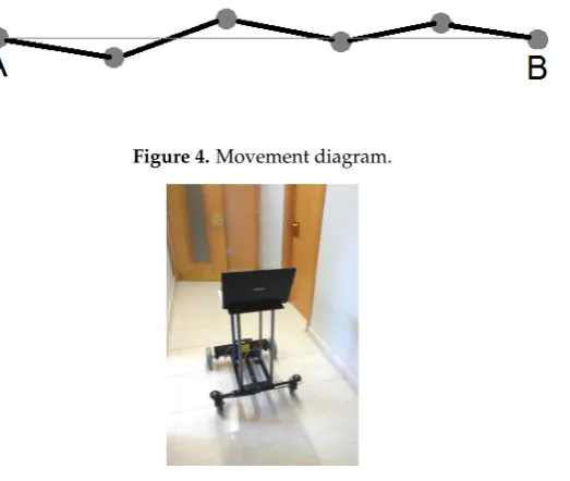
The movement of the robot while trying to travel in a straight line is ilustrated in Fig. 4. The
79
actual distance from A to B is not the output of the encoder corrected by the conversion factorcm. 80
However, if the robot’s orientation is kept below a given threshold, the maximum deviation of that
81
measurement can be controlled. For example, if the orientation remains below 1◦, then the maximum
82
deviation remains less than 0.02%, and for 2◦, less than 0.06%. Those deviations can be accepted for
83
our experiments and we will analyse the robot’s orientation to reject those measurements where the
84
maximum deviation of orientation has been greater than a given threshold.
85
The right wheel is taken as a reference, and DL is corrected by the factor Ed. In the second experiment, a straight motion for 3 m is performed by the robot, and the number of pulses of the right wheel,P2R, with the actual distance traveledd3mgives the conversion factor from pulses to mm as
cm= d3m P2R
The actualDRis given by
DR= cmce
π (2)
in our case,ce =152.7 pulses/rev. 86
Coming back to Equation (1), the actualbis given by
bact= P1RDR
2ce andEsis obtained as the mean ofDRandDL:
Es= DR
Dnom 1+Ed
2 (3)
We found a problem with the effective wheelbase (be f f). It is larger when the speed–wheel relation 87
is close to unity, and is smaller when one of the wheels is stopped. Most of the movements during
Figure 4.Movement diagram.
Figure 5.Robotic platform.
the robot’s operation are performed with the two wheels having similar speeds, but the proposed
89
calibration method uses part of the experiments with one wheel stopped.
90
In order to getbe f f, we performed a movement turning over one stopped wheel and then turning with both wheels at the same speed, taking into account the number of pulses to complete a turn with the stopped wheelP0Rb and the number of pulses when turning with the two wheels at the same speed
P0Rb
/2. Then, the factor to obtainbe f f is
K= 2
∗P0Rb/2
P0Rb
3. Experiments 91
Our robot software has 3 parameters to adjust. They are set before starting each calibration method:
cm= πDnom ce
= π190
157.2 =3.80 mm/pulse
Ed=1 and
b=590 mm 3.1. UAH Calibration 1
92
The first experiment was carried out with the robot platform shown in Fig.5. First, we obtained the effective wheelbase factor for movements with a stopped wheel, so the robot performed movements as was explained previously. We getP0Rb =951 pulses andP0Rb/2 =478 pulses, so
K=1.0053.
Then, with the left wheel stopped, the robot performed a given number of rounds and the
93
experiment was then repeated for a stopped right wheel.
94
Fig.6shows the output of the ultrasound sensor for 7 turns and in Fig.7just 2 periods are plotted.
95
It is important to be sure that the scenario is not symmetrical in order to get the proper period. In
96
our case, because of the limited sensor range, the scenario must not be very large. Fig.8shows the
Figure 6.Sensor Output rotating over the left wheel.
Figure 7.Zoom Sensor Output over the left wheel. Table 1.Results from the second experiments
Iteration P2R distance max(θ) cm (Pulses) (mm) (degrees) (mm/pulse)
1 795 3078 0.75 3.87
2 795 3068 0.93 3.86
3 795 3068 0.75 3.86
4 795 3070 0.76 3.86
autocorrelation sequence of the sensor output and from this data the period, i.e. the number of pulses
98
per turn, can be easily obtained.
99
The number of pulses when the left wheel is stopped per turn (period)P1R is
P1R ={951.1, 952.0, 951.0} pulses
for three iterations, as can be seen the variance for different iterations is low. When the right wheel is stopped,P1L is
P1L ={944.0, 943.0, 943.0} pulses
also for three iterations of the experiment. So, taking the mean value
Ed= DL
DR = P1R
P1L
=1.007
Now, in order to perform the second experiment, theEdfactor must be included in the robot’s 100
odometry, so we set up the newEdin the robot software or automatically update it if the calculation is 101
done on-board.
102
Then a 3m long motion is performed and the number of pulses in several iterations are illustrated
103
in Table1, where the number of pulses for the distance actually travelled gives the factorcm. The 104
maximum deviation in orientation is also considered in order to discard those results with deviations
105
bigger than 1◦.
106
Figure 8.Sensor output autocorrelation sequence.
The wheelbase distancebcan be obtained from 2πb=P1R·cm
butP1Rwas obtained from a movement with stopped left wheel, so it must be corrected withK:
2πb
K =P1R·cm
so,b = 951.3·3.862 ·1.0053
π = 586.5 mm, from Equation (2) DR = 187.61 mm and from Equation (3) 108
Es = 0.9924 where the used nominal diameter was Dnom = 190 mm and the new avarage of the 109
diameters isDavg =188.55 mm. We do not useDavgbut it will be necessary to perform a calibration 110
from [1] for comparison.
111
3.2. UMB Calibration 112
TheDavgfrom UAH calibration 1 is used to perform the UBM calibration [1]. The setup parameters are
cm= πDnom
ce
= π188.55 152.7 =3.88
Ed=1 and
b=590.
The UMB method [1] was carried out for a square of L = 2 m (as was suggested in [5]) for 5
113
rounds clockwise and 5 counterclockwise, writing the final point deviations of each movement. Our
114
robot platform is almost 1 m long and a larger free scenario was not viable.
115
The results for the error centres of gravity for clockwise (Xcg,cw,Ycg,cw) and counterclockwise (Xcg,ccw,Ycg,ccw) are
Xcg,cv/ccw= 1 5
5
∑
i=1
exi,cv/ccw
Ycg,ccw= 1 5
5
∑
i=1
eyi,cv/ccw
where the error is the difference between the actual absolute position of the robot and the calculated one.
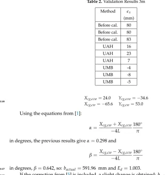
Before cal. 80 Before cal. 80 Before cal. 83
UAH 16
UAH 23
UAH 7
UMB -4
UMB -8
UMB -5
Xcg,ccw=24.0 Ycg,ccw=−34.6 Xcg,cw=−65.6 Ycg,cw=53.0
116
Using the equations from [1]:
α= Xcg,cw
+Xcg,ccw −4L
180◦
π
in degrees, the previous results giveα=0.298 and
β= Xcg,cw
−Xcg,ccw −4L
180◦
π
in degrees,β=0.642, so:bactual=591.96 mm andEd=1.003. 117
If the correction from [5] is included, a slight change is obtained:bactual=591.98 mm. 118
4. Validation 119
In [1], the same experiment used for calibration is repeated after calibration in order to test the
120
method. The distances from zero error to the centres of gravity are used to compare the results. This
121
validation process needs a large space to perform the test. In [4] and [3], only simulation results are
122
presented to compare the methods.
123
Table2shows the error in the first 3 m of the experiment, and Table3the error after the whole
124
journey.
125
To validate the results of calibration, travelling along a 3 m long path, followed by a turn through
126
an angle of π and then coming back again 3 m, was carried out. Table2and 3show the error 127
(ex =xabs−xcalcandey = yabs−ycalc) in mm in theXandYcoordinates before calibration for the 128
calibration method UAH and for UMBmark. Table2after the first 3 m of travel and Table3after
129
coming back.
130
The tests were been performed 3 times for each calibration in order to avoid non-systematic error.
131
Note that the error in Table2comes bassically from the error in the wheel diameters and the error in
132
Table3is affected by the wheel diameters andb.
133
Fig.9shows the error before calibration, with the UMB method calibration and the proposed one.
134
As can be seen, the results for both calibrations are very similar, although sligthly better for the UMB
135
method. But the simplicity of our method leads us to use it instead of the UMB. It must be taken into
136
account that most of the measurements in the proposed method are done on-board and in most of the
137
movements, the initial point is not important.
Table 3.Validation Results 3m-π-3m
Method ex ey
(mm) (mm) Before cal. 109 223 Before cal. 98 273 Before cal. 95 248
UAH 1 71 36
UAH 1 78 -17 UAH 1 71 -24
UMB 72 -4
UMB 71 21
UMB 76 17
Figure 9.Error from different calibrations.
5. Conclusions 139
A new method for differential drive robot calibration has been presented. One of the main
140
contributions is that free space needed to perform the calibration in our method is very small. Another
141
feature to point out is that the number of manual measurements is just one with our method, which
142
can be repeated in order to check the correctness, but checking the maximum orientation makes it easy
143
to discard wrong measurements. The most complicated part of the calibration method can be done
144
on-board. If a calibrated distance sensor is available, the whole method can be implemented on-board.
145
The results are very close to those obtained with the UMB method, so we use our method instead
146
because of its simplicity in performing the calibration.
147
Funding:This work was partially supported by the University Alcala research program through the projects 148
CCG2016/EXP-045 and CCG2016/EXP-042 and TEC2016-80326-R from the “Ministerio de Economíía, Industria y 149
Competitividad”. 150
Author Contributions:All authors contributed equally to this work. 151
Conflicts of Interest:The authors declare that there are no conflicts of interest regarding the publication of this 152
paper. 153
References 154
1. J. Borenstein and L. Feng, “Correction of systematic odometry errors in mobile robots,” inIntelligent Robots
155
and Systems 95.’Human Robot Interaction and Cooperative Robots’, Proceedings. 1995 IEEE/RSJ International
156
Conference on, vol. 3. IEEE, 1995, pp. 569–574.
pp. 2073–2078. 162
4. A. Bostani, A. Vakili, and T. A. Denidni, “A novel method to measure and correct the odometry errors in 163
mobile robots,” inElectrical and Computer Engineering, 2008. CCECE 2008. Canadian Conference on. IEEE, 164
2008, pp. 000 897–000 900. 165
5. K. Lee, C. Jung, and W. Chung, “Accurate calibration of kinematic parameters for two wheel differential 166
mobile robots,”Journal of mechanical science and technology, vol. 25, no. 6, p. 1603, 2011. 167
6. A. Martinelli, N. Tomatis, and R. Siegwart, “Simultaneous localization and odometry self calibration for 168