https://doi.org/10.5194/nhess-18-65-2018 © Author(s) 2018. This work is distributed under the Creative Commons Attribution 3.0 License.
Detection of collapsed buildings from lidar data due to the 2016
Kumamoto earthquake in Japan
Luis Moya1, Fumio Yamazaki2, Wen Liu2, and Masumi Yamada3
1International Research Institute of Disaster Science, Tohoku University, Miyagi, Sendai, 980-0845, Japan 2Department of Urban Environment Systems, Chiba University, Chiba 263-8522, Japan
3Disaster Prevention Research Institute, Kyoto University, Gokasho, Uji, 611-0011, Japan Correspondence:Luis Moya (lmoyah@irides.tohoku.ac.jp)
Received: 26 May 2017 – Discussion started: 19 June 2017
Revised: 20 November 2017 – Accepted: 20 November 2017 – Published: 4 January 2018
Abstract. The 2016 Kumamoto earthquake sequence was triggered by anMw6.2 event at 21:26 on 14 April. Approxi-mately 28 h later, at 01:25 on 16 April, anMw7.0 event (the mainshock) followed. The epicenters of both events were lo-cated near the residential area of Mashiki and affected the re-gion nearby. Due to very strong seismic ground motion, the earthquake produced extensive damage to buildings and in-frastructure. In this paper, collapsed buildings were detected using a pair of digital surface models (DSMs), taken before and after the 16 April mainshock by airborne light detection and ranging (lidar) flights. Different methods were evaluated to identify collapsed buildings from the DSMs. The change in average elevation within a building footprint was found to be the most important factor. Finally, the distribution of collapsed buildings in the study area was presented, and the result was consistent with that of a building damage survey performed after the earthquake.
1 Introduction
The detection of affected areas after an earthquake is very im-portant for disaster response activities. Allocating resources such as relief forces, food, medicine, and shelter is crucial af-ter a natural disasaf-ter strikes (Das and Hanaoka, 2014). Thus, proper information on the damage situation will improve the efficiency of distributing relief resources. The extent of the affected area also provides an idea of the scale of the disaster and an estimate of the relief demand. Damage assessment af-ter an earthquake disasaf-ter is important for the scientific com-munity as well. A significant amount of information has been
obtained from previous earthquakes and used to improve construction design codes to evaluate and mitigate damage to buildings and infrastructure in the event of future quakes. For instance, Whitman et al. (1973) provided earth-quake damage probability matrices using data collected after the 1971 San Fernando, California earthquake. Yamazaki and Murao (2000) proposed vulnerability functions for Japanese buildings based on building inventory and damage data and the spatial distribution of strong motion (Yamaguchi and Ya-mazaki, 2001) during the 1995 Kobe earthquake in Japan.
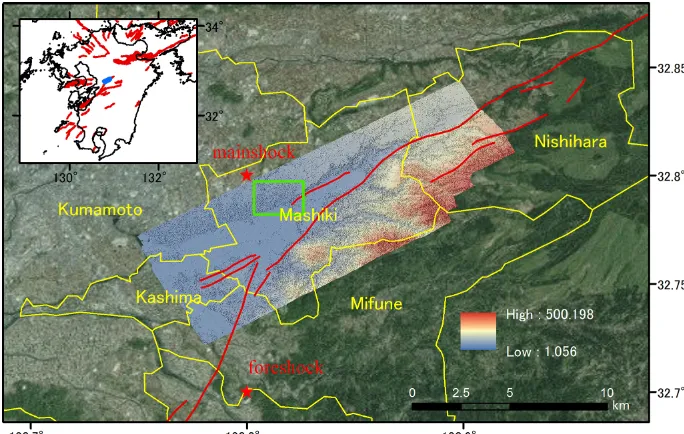
Figure 1.The post-event lidar data for the study area. Shaded colors represent the elevation. The green rectangle shows the locations of the area surveyed by Yamada et al. (2017). The inset shows Kyushu Island, and the blue polygon in the inset depicts the study area.
Schweier and Markus (2006) pointed out that airborne light detection and ranging (lidar) data can be used to classify collapsed buildings using the following geometrical features of a building extracted from lidar data: the height change from the initial one, the reduction of the total volume, the footprint borders, the inclination of the structure, the debris spread outside the footprint, the additional covered area out-side the footprint, and the damage situation of the roof. They proposed a modification of the previous damage classifica-tion method (Okada and Takai, 2000) using these geomet-rical features. Although they suggested the use of airborne lidar data to analyze collapsed buildings, applications to real cases were not provided.
Applications of lidar for damage detection are still few compared with other remote-sensing technologies. The main reason is the lack of lidar data before a disaster. However, Aixia et al. (2016) performed a study on the possibility of detecting building damage using only a post-earthquake li-dar digital surface model (DSM). Their results are promising for buildings with simple roof shapes, such as flat and pitched roofs. Rehor et al. (2008) proposed the use of a plane-based segmentation method to detect damaged buildings, wherein the number of unsegmented pixels in damaged buildings is larger than in undamaged buildings. Labiak et al. (2011) pro-posed an automated method to detect and quantify building damage using only a post-earthquake lidar DSM as well, but their results had low accuracy for heavily damaged and col-lapsed buildings. Hussain et al. (2011) combined lidar data with GeoEye-1 imagery to detect damaged buildings after the 2010 Haiti earthquake. They detected 190 damaged build-ings out of 200; however, their procedure required manual intervention, and the damage level was not clearly classified.
Instead of lidar data, Maruyama et al. (2014) constructed two DSMs from two sets of aerial images: before and after the earthquake. Then, the collapsed buildings after the 2007 Niigata-Chuetsu-Oki earthquake, Japan, were identified us-ing the difference in elevation between the DSMs.
An Mw6.2 earthquake struck Kumamoto Prefecture, Japan, on 14 April 2016 at 21:26 JST. The event pro-duced structural damage and resulted in nine human casu-alties (Cabinet Office of Japan, 2017). Then, 28 h later, a second earthquake withMw7.0 occurred close to the first one. Thus, the first event was designated the “foreshock” and the second the “mainshock”. The epicenter of the foreshock was located at the end of the Hinagu fault, and the epicenter of the mainshock was located in the Futugawa fault. Both events were located in the town of Mashiki, which has a population of 33 000. The number of aftershocks following these events reached the largest number among recent inland earthquakes in Japan (Japan Meteorological Agency, 2017). The total number of deaths due to direct causes reached 50, and over 8000 residential buildings were severely damaged or collapsed due to the Kumamoto earthquake sequence.
devia-tion, and the correlation coefficient are tested for this pur-pose.
2 Study area and data set
After the foreshock, a lidar-surveying flight was carried out during 15:00–17:00 (JST) on 15 April 2016 in order to record the effects of the earthquake (Asia Air Survey Co., Ltd., 2017). It produced point clouds with an average point density of 1.5–2 points m−2. Subsequently, because the unexpected mainshock occurred, a second mission was set up during 10:00–12:00 (JST) on 23 April 2016, which produced point clouds with an average point density of 3–4 points m−2. Both sets of lidar data were acquired using a Leica ALS50II instru-ment and the same pilot and airplane. After rasterization of the raw point clouds, two DSMs with a data spacing of 50 cm were created. The DSMs collected before and after the main-shock will hereafter be referred to as the BDSM and ADSM. Figure 1 shows the extent of the ADSM, which represents the entire study area. It covers the main part of Mashiki and some parts of Nishihara village, Mifune and Kashima towns, and Kumamoto city.
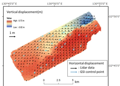
The study area is located in the near field of the Kumamoto earthquake sequence where significant permanent ground displacements were produced during the earthquake. A direct comparison of the BDSM and ADSM shows that the build-ing coordinates do not match because the ADSM contains coseismic displacements. Therefore, the ADSM was shifted before detecting the damaged buildings based on the per-manent crustal movement calculated by Moya et al. (2017). To do this, an automated procedure for calculating the per-manent three-dimensional (3-D) displacement was imple-mented. The permanent ground displacement was calculated by 100 m grid size and then applied to the ADSM pixels within the grid size. Figure 2 illustrates the calculated per-manent ground displacement of the common lidar data area. In the figure, the results of new field measurement carried out in August 2016 for surveying reference points after the Kumamoto earthquake are also shown (Geospatial Informa-tion Authority of Japan, 2017). The coseismic displacements estimated from the lidar data show good agreement with the survey results (Fig. 3). In Fig. 2, the causative fault is located in the areas where sudden changes in the direction of the per-manent ground displacement are observed. Over the entire study area, a maximum horizontal displacement of approxi-mately 2 m was observed.
3 Detection of damaged buildings
To focus on buildings, a geocoded building footprint data set, provided by the Geospatial Information Authority of Japan (GSI), was used. Only buildings with footprint areas greater than 20 m2were evaluated. Because the point densi-ties of the BDSM and ADSM are different and the footprint
Figure 2.Estimated three-dimensional coseismic displacement af-ter the mainshock of the 2016 Kumamoto earthquake. The black arrows and the shaded colors indicate the horizontal and vertical displacements obtained from lidar (Moya et al., 2017). The blue arrows indicate the horizontal displacements at the control points measured by the Geospatial Information Authority of Japan (2016).
Figure 3.Comparison between the coseismic displacements esti-mated from the lidar data (Moya et al., 2017) and from field mea-surements (Geospatial Information Authority of Japan, 2016).
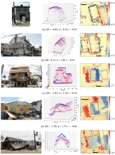
data include some errors, perfect matching of the DSMs with the building footprints could not be achieved. For this rea-son, the building footprints were reduced by 1 m (i.e., the reduced polygon is located inside a building footprint), and they were projected onto the same reference system as that of the DSMs (Fig. 4). The lidar data within the reduced build-ing boundaries were then extracted and processed. The rea-son for using the reduced building boundaries was to discard the DSM data near the building boundaries in the subsequent analysis. The distance of the buffer (1 m) was decided based on a preliminary evaluation of the data (Moya et al., 2016).
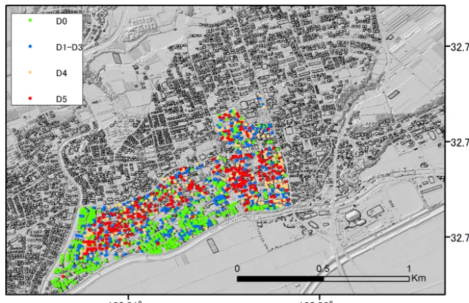
Figure 5.Building damage survey data from Yamada et al. (2017). The location of the survey area is shown in Fig. 1.
ues around the boundary of the building footprint, which was caused by the effect mentioned earlier. These errors are cer-tainly present for tilted buildings as well and make damage detection very challenging (Fig. 4b). Figure 4c shows a typi-cal collapsed steel-frame building with a well-known damage pattern that occurs with a soft story or a weak story, that is, a significant difference in the stiffness/resistance between one story and the rest. They show a significant horizontal/vertical movement, which is easier to detect by lidar data. Figure 4d shows a collapsed wooden building that was shifted signifi-cantly in the horizontal direction. Conversely, the collapsed wooden building shown in Fig. 4e does not exhibit a horizon-tal movement, only a vertical shift. Lateral spread of debris is an important issue when the building is located along a main road. For almost all the collapsed buildings, a clear decrease in building elevation was observed from the lidar DSMs.
The number of buildings within the study area is very large, so it is necessary to implement an automated procedure to evaluate the extent of their damage. In this study, three pa-rameters were used: the average height difference between the two DSMs (1H )within the reduced building footprint, its standard deviation (σ ), and the correlation coefficient (r) between the two DSMs. These parameters were calculated for each building using the following equations:
1H= 1 N
N X
i=1
(Hai−Hbi) (1)
σ = v u u u t N P
i=1
((Hai−Hbi)−1H )2
N (2)
r= (3)
N N P
i=1
HaiHbi− N P
i=1 Hai
N P
i=1 Hbi v u u t N N P
i=1 Ha2i −
N P
i=1 Hai
2! N
N P
i=1 Hb2i −
N P
i=1 Hbi
2!
where i∈ {1,2, . . ., N} and N is the number of elevation points inside a given reduced building footprint. Haiand Hbi are the elevations from the ADSM and BDSM. The correla-tion coefficient ranges from−1.0 to 1.0 and has proven to be effective in detecting changes from a pair of satellite im-ages (Liu et al., 2013; Uprety et al., 2013). A value ofrclose to 1.0 indicates no change.
Yamada et al. (2017) presented the distribution of build-ing damage in the central part of Mashiki, wherein the dam-age was determined from aerial photos and field surveys. The damaged buildings were classified into four categories: no damage (D0), partial/moderate damage (D1–D3), severe damage/incline (D4), and story collapse (D5). Here, D1– D5 represent the degree of damage according to Okada and Takai (2000), which is similar to G1–G5 of the European Macroseismic Scale (EMS-98). Figure 5 shows the damage distribution over the surveyed area, which is located along the north side of the Akitsu River.
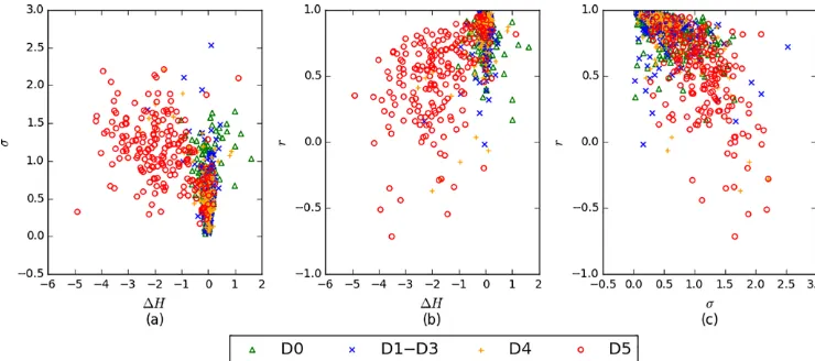
Figure 6.Scatter plots of the three parameters (1H,σ,r)calculated from the lidar DSMs for the buildings surveyed by Yamada et al. (2017).
observed regardless of which parameter was chosen. On the other hand, collapsed buildings (D5) tend to have large neg-ative values of1H. Therefore, this paper focuses on the de-tection of collapsed buildings. It is important to note that few collapsed buildings show positive values of 1H. A closer look showed that those buildings were covered by a neigh-boring building that had collapsed.
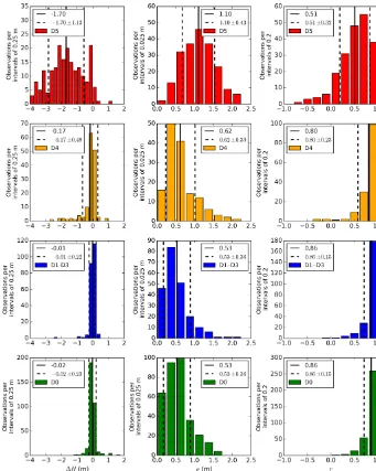
Although 1H seems to be the dominant parameter for identifying collapsed buildings, the other two parameters (σ andr)can still provide additional information. For instance, if we observe the collapsed buildings from the scatter plot in Fig. 6c (red marks), a trend can be observed in which r trends to one whenσ is close to zero. This trend is related to the collapse patterns and can be observed for the collapsed buildings shown in Fig. 4. Figure 4d shows a completely col-lapsed building in which the debris has spread laterally. For those cases, the values ofr are low and the values ofσ are large. On the other hand, Fig. 4e shows a collapsed build-ing with a roof that remained almost the same shape while it collapsed almost vertically. This means that all the elevations inside the footprint decreased by about the same amount, thus leading to a high value ofrand a low value ofσ. This pattern is often difficult to detect from optical aerial and satellite op-tical images, because the sensor measures the landscape ver-tically. The histograms for collapsed buildings (Fig. 7) shows that several collapsed buildings have a value for r greater than 0.5, and it would be difficult to detect this from aerial or optical satellite imagery. Readers might notice that noncol-lapsed buildings also have a value ofrclose to 1 andσclose to zero; however, those can be first filtered using1H.Then, the pattern of collapse can be evaluated from the other two parameters (using a decision tree).
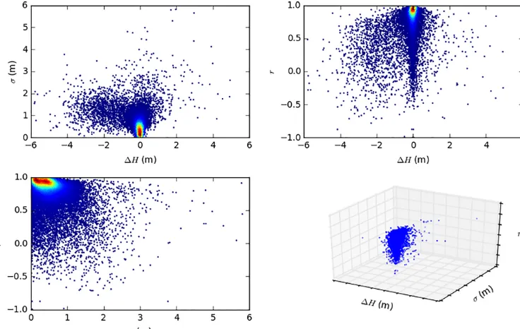
Within the study area, 26 128 building footprints were found. It is worth mentioning that few buildings were not well registered in the GIS map. Figure 8 shows the param-eters calculated for each building, wherein the shaded color depicts the density of the dots. Most of the points are
lo-cated at approximately (1H,σ,r)=(0 m, 0.5 m, 0.9), which indeed represents noncollapsed buildings. Several buildings show positive values of 1H. A closer look revealed two principle factors: (1) the collapse of a neighboring building and (2) plastic covers placed over the roof for protection from the rain.
The next concern was to define a criterion to set threshold values that can differentiate collapsed/noncollapsed build-ings properly. A number of options were evaluated in this study. Since it is obvious that the buildings with clear nega-tive values of1Hcorrespond to collapsed buildings, we first analyzed the classification using a threshold for 1Honly. The buildings with 1Hvalues smaller than that threshold were classified as collapsed; the buildings with1H values greater than the threshold were classified as noncollapsed. The possible thresholds were tested on the buildings sur-veyed by Yamada et al. (2017). Figure 9 shows the Cohen’s kappa coefficient and the overall accuracy calculated from the comparison between the estimated collapsed and non-collapsed buildings (i.e., using a given threshold) and the building damage classes based on the ground truth. For the comparison, the buildings with damage levels D0, D1–D3, and D4 were labeled noncollapsed buildings. The Cohen’s kappa (k)coefficient and the overall accuracy (OA) are ex-pressed as follows:
pno=(p21+p22)(p12+p22) (4)
pyes=(p11+p12)(p11+p21) (5)
po=p11+p22 (6)
pe=pyes+pno (7)
OA=po (8)
k=po−pe 1−pe
, (9)
noncol-Figure 7.Histograms of the three parameters (1H,σ,r)calculated from the lidar DSMs for the buildings surveyed by Yamada et al. (2017), separated into four damage levels.
lapsed and collapsed buildings. From Fig. 9, it is observed that a threshold value of−0.5 m gave the highest values for both the Cohen’s kappa coefficient (0.80) and the overall ac-curacy (0.93).
To determine whether the use of all the parameters could produce better accuracy in detecting collapsed buildings, the support vector machine (SVM) method was selected to construct a plane that separates collapsed and noncollapsed buildings in the three-dimensional database (1H, σ, r). The plane has the largest distance from the nearest train-ing data (ground truth data). Ustrain-ing kernel functions, SVM can be used to construct a nonlinear function as well. How-ever, in this study we only evaluated linear functions (i.e., a plane or linear kernel function). Figure 10 shows the plane
Figure 8.Scatter plots of the three parameters (1H,σ,r)calculated for all the buildings in the study area. The color represents the density of points, wherein red shows the area with the highest density.
Figure 9.Kappa coefficient(a)and overall accuracy(b)obtained from the comparison between the data surveyed by Yamada et al. (2017) and the estimated collapsed buildings based on different
1H threshold values.
expression:
w=X i
αiyixi, (10)
wherexiis a training vector that contains the three parame-ters (1H,σ andr),yi represents the class that can be either 1 or−1, and the coefficientsαi are obtained by solving the following problem:
min α
1 2α
TQα−eTα
(11)
Qij=yiyj xi·xj (12)
0≤αi ≤C, i=1, . . ., n, (13)
whereeis a vector with elements that are all ones.Cis the upper bound and is used as a regularization parameter.
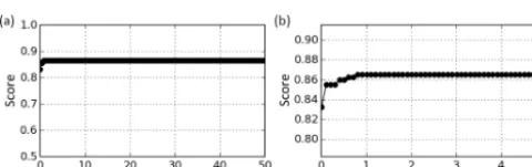
The parameterC trades off misclassification of training examples against simplicity of the decision surface. A low C value makes the decision surface smooth and a high C value aims to classify all training examples correctly (Skit-learn, 2017a). In this study a valueCequals to 1 was used. In order to evaluate its effects, a cross-validation procedure was performed. For eachCvalue, 80 % of the surveyed data were selected randomly and were used to calibrate the SVM classifier. The rest of the surveyed data were used to calculate a score that represents the accuracy. The overall accuracy was chose as the score. The procedure was repeated five times and the average was stored. Figure 11 shows the cross-validation accuracy. It is observed the accuracy remains mainly constant with small fluctuations at lower values. However, a difference of approximately 3 % is observed between the worst and the best accuracy. Therefore, it is concluded that theCvalue did not affect the SVM classifier in our study.
Figure 10.Classification of collapsed (red) and noncollapsed (blue) buildings using the three parameters based on SVM.
Figure 11.The classifier’s cross-validation accuracy as a function ofC.(a)Overall evaluated range ofC.(b)A closer look at values lower than 5.
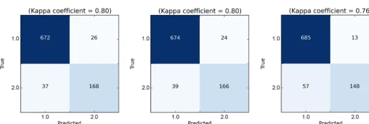
distance from each other (Scikit-learn, 2017b). Figure 12 rep-resents the predicted collapsed and noncollapsed buildings using thek-means clustering method, for which the Cohen’s kappa coefficient obtained was 0.76. Figure 13 shows the confusion matrix calculated from the comparison between the ground truth data and the predicted results from the three methods explained above, applying a1H threshold, SVM, andk-means clustering. The first two methods show the same level of accuracy, whilek-means clustering shows a lower ac-curacy.
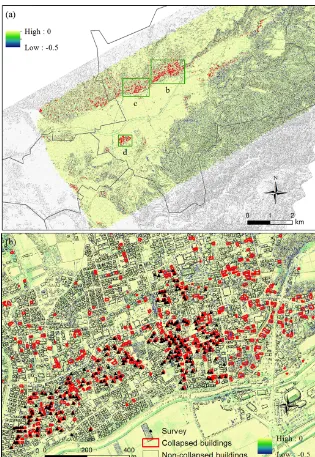
Figure 14 illustrates the spatial distribution of collapsed buildings estimated using a1Hthreshold of−0.5 m. A large number of collapsed buildings were observed in the study area (Fig. 14a). The red and black polygons represent the collapsed (D5) and noncollapsed (D0–D4) buildings. The color of the pixels represents the difference in elevations be-tween the ADSM and BDSM. Blue pixels depict differences of elevations less than−0.5 m, and yellow pixels represent differences greater than 0 m. Figures 14b and 15 provide a closer look of the areas where the collapsed buildings are concentrated. Figure 14b also depicts the location of the col-lapsed buildings surveyed by Yamada et al. (2017) as black triangles. Within the study area, a total of 26 128 buildings were evaluated, and 1760 buildings were classified as col-lapsed (1H less than−0.5 m).
It was observed that some buildings that collapsed dur-ing the foreshock (14 April event) were also detected by the lidar methods. In order to be detected, the debris of those buildings should be either severely disturbed by the main-shock (16 April event) or removed before the ADSM was
recorded. For instance, Fig. 16 shows two buildings that col-lapsed during the foreshock (Fig. 16a). However, because the mainshock produced a significant reduction in their eleva-tions (Fig. 16b), it was also detected from the pair of lidar.
4 Discussion
This paper evaluated the use of lidar data to detect dam-aged buildings by means of three parameters:1H,σ, and r. It was found that collapsed buildings can be identified pre-cisely from the average difference in height,1H. However, the other two parameters can provide additional information about the collapse pattern. The collapsed patterns are corre-lated with the failure mechanism of buildings, which might highlight some deficiencies in the design codes that were used in the construction process. A detailed understanding of the failure mechanism is important to the practice of foren-sic engineering, the investigation of failures and other per-formance problems. Moreover, with further evaluation, the collapsed pattern might contribute to future improvements of the building design codes. Unfortunately, it was not possi-ble to calibrate a threshold that can properly classify differ-ent collapsed patterns. The main reason is because there was no information related to the collapse patterns in the survey data. Perhaps this task can be done in future research after new survey data are released.
Figure 13. Confusion matrix calculated from the comparison of the ground truth data and the predicted damage levels based on the
1Hthreshold(a), SVM(b), andk-means clustering(c). Two damage levels, noncollapsed (1.0) and collapsed (2.0), were employed.
the data set. However, the authors decided to work with the data in its current state because this uncertainty is likely to be present in other real situations in which a quick report on damage extent is required.
Of the three methods evaluated here, thek-means cluster-ing exhibits the lowest accuracy. The main reason is that, un-like the SVM method, the k-means clustering does not use any truth data. However, it produced a kappa coefficient of 0.76 and overall accuracy of 92 %, which is still quite good. The k-means clustering method is useful for taking a first glance at the distribution of collapsed buildings because the method does not require any training data. The procedure is well-known and robust, with several efficient algorithms with proven fast convergence.
Finally we would like to discuss the building damage rate in the Kumamoto earthquake in comparison to other recent M7-level crustal earthquakes in Japan. In the 1995 Kobe earthquake (Mw6.9), about 49 000 buildings were col-lapsed (G5 in EMS-98 scale) or severely damaged (G4) out of 560 000 buildings in the affected urban area (Building Re-search Institute, 1996). The recorded strong motion distri-bution in the Kobe earthquake was at a similar level to that of the Kumamoto earthquake (Yamaguchi and Yamazaki, 2001). However, in 1995, the number of strong motion ac-celerometers was much lower, about only 10 in the hard-hit zone. The building density of the affected area was much
higher in the Kobe region than that of the Kumamoto re-gion. Considering these differences, it is difficult to con-clude which earthquake was more destructive. From our experiences (Yamazaki and Murao, 2000; Yamaguchi and Yamazaki, 2000), the severity of damage for timber-frame houses in Mashiki was at a similar level to that in the hard-hit zone of the Kobe region. There were a few more recent M7-level crustal earthquakes in Japan, such as the 2004 Niigata-Chuetsu earthquake (Mw6.6) and the 2007 Niigata-Chuetsu-Oki earthquake (Mw6.6). However, the population density of the affected urban areas was lower in these events, and thus it is again difficult to compare their damage situations (Nagao et al., 2011) with that of Kumamoto, although their strong motion levels were again comparable with that of the Ku-mamoto event.
main-Figure 14. (a) A map showing the distribution of collapsed (1H <−0.5 m) buildings, shown as red polygons, in the study area. The pixel color represents the difference in elevation between the BDSM and ADSM. The green squares show the locations of areas shown in panel(b)and Fig. 15. Close-up view of area(b)in which the collapsed buildings were concentrated. The black triangles show the D5 buildings from Yamada et al. (2017).
shock excitations. More detailed results on this matter will be presented in the near future.
5 Conclusions
In this study, the spatial distribution of collapsed buildings was extracted from a pair of lidar data sets taken before and after the 2016 Mw7.0 Kumamoto earthquake. For this pur-pose, geographic information on building footprints was em-ployed. Three parameters were used: the average (1H )and
Figure 15.Close-up view of areas(c)and(d)in Fig. 14a where collapsed buildings are concentrated. The red and green polygons are the collapsed and noncollapsed buildings estimated using the threshold (1H <−0.5 m).
Figure 16. (a)Aerial image taken on 15 April;(b) aerial image taken on April 23. The thick red polygons show buildings that col-lapsed after the foreshock and were detected using the1H thresh-old.
was illustrated together with the height difference between the two DSMs, and good agreement was observed. From a total of 26 128 evaluated buildings, 1760 collapsed buildings were identified. To our knowledge, this result may be the first case in which a large number of collapsed buildings were identified from a pre- and post-event lidar DSM pair.
Data availability. The digital surface models used in this study are owned and provided by Asia Air Survey Co., Ltd. The building foot-print data are available from the website of the Geospatial Informa-tion Authority of Japan.
Competing interests. The authors declare that they have no conflict of interest.
Acknowledgements. This study was financially supported by a Grant-in-Aid for Scientific Research (project numbers: 17H02066, 24241059) and the Core Research for Evolutional Science and Technology (CREST) program by the Japan Science and Tech-nology Agency (JST) “Establishing the most advanced disaster reduction management system by fusion of real-time disaster simulation and big data assimilation (Research Director: Shu-nichi Koshimura of Tohoku University)”.
Edited by: Oded Katz
Reviewed by: two anonymous referees
References
Aixia, D., Zongjin, M., Shusong, H., and Xiaoqing, W.: Building damage extraction from post-earthquake airborne LiDAR data, Acta Geol. Sin.-Engl., 90, 1481–1489. 2016.
Asia Air Survey Co., Ltd.: The 2016 Kumamoto earthquake, avail-able at: http://www.ajiko.co.jp/article/detail/ID5725UVGCD/, last access: 1 April 2017.
Building Research Institute: Final report of damage survey of the 1995 Hyogoken-Nanbu earthquake, available at: http://www.kenken.go.jp/japanese/research/iisee/list/topics/ hyogo/pdf/h7-hyougo-jp-all.pdf (last access: 1 September 2017), 1996 (in Japanese).
Building Research Institute: Wallstat version 3.1, collapsing sim-ulation program for timber structures, available at: http:// www.nilim.go.jp/lab/idg/nakagawa/wallstat.html (last access: 1 September 2017), 10 September 2015.
Cabinet Office of Japan: Summary of damage situation in the Ku-mamoto earthquake sequence, available at: http://www.bousai. go.jp/updates/h280414jishin/index.html, last access: 1 Septem-ber 2017 (in Japanese).
Das, R. and Hanaoka, S.: An agent-based model for resource alloca-tion during relief distribualloca-tion, Journal of Humanitarian Logistics and Supply Chain Management, 4, 265–285, 2014.
Dell’Acqua, F. and Gamba, P.: Remote sensing and earthquake damage assessment: Experiences, limits, and perspectives, Pro-ceedings of the IEEE, 100, 2876–2890, 2012.
Geospatial Information Authority of Japan: New measure-ment for survey reference points after the 2016 Kumamoto Earthquake, available at: http://www.gsi.go.jp/sokuchikijun/ sokuchikijun60019.html, last access: 1 April 2017.
Hashemi-Parast, S. O., Yamazaki, F., and Liu, W.: Monitoring and evaluation of the urban reconstruction process in Bam, Iran, after the 2003Mw6.6 earthquake, Nat. Hazards, 85, 197–213, 2017. Hoshi, T., Murao, O., Yoshino, K., Yamazaki, F., and Estrada, M.:
Post-disaster urban recovery monitoring in Pisco after the 2007
Peru earthquake using satellite image, Journal of Disaster Re-search, 9, 1059–1068, 2014.
Hussain, E., Ural, S., Kim, K., Fu, C., and Shan, J.: Building extrac-tion and rubble mapping for city Port-au-Prince post-2010 earth-quake with GeoEye-1 imagery and Lidar Data, Photogramm. Eng. Rem. S., 77, 1011–1023, 2011.
Japan Meteorological Agency: The number of aftershocks of re-cent inland earthquakes in Japan, http://www.data.jma.go.jp/svd/ eqev/data/2016_04_14_kumamoto/kaidan.pdf, last access: Jan-uary 2017 (in Japanese).
Korosov, A. A., Hansen, M. W., Dagestad, K., Yamanaka, A., Vines, A., and Riechert, M.: Nansat: a scientist-orientated python pack-age for geospatial data processing, Journal of Open Research Software, 4, 11 pp., 2016.
Labiak, R. C., Aardt, J. A. N., Bespalov, D., Eychner, D., Wirch, E., and Bischof, P.: Automated method for detection and quan-tification of building damage and debris using post-disaster Lidar data, Proc. SPIE 8037, Laser Radar Technology and Applications XVI, Vol. 8037, 8 pp., 2011.
Liu, W., Yamazaki, F., Gokon, H., and Koshimura, S.: Extrac-tion of tsunami-flooded areas and damaged buildings in the 2011 Tohoku-oki earthquake from TerraSAR-X intensity images, Earthq. Spectra, 29, S183–S200, 2013.
Maruyama, Y., Tashiro, A., and Yamazaki, F.: Detection of col-lapsed buildings due to earthquakes using a digital surface model constructed from aerial images, J. Earthq. Tsunami, 8, 1450003 (13 pp.), 2014.
Meslem, A., Yamazaki, F., and Maruyama, Y.: Accurate evaluation of building damage in the 2003 Boumerdes, Algeria earthquake from Quickbird satellite images, J. Earthq. Tsunami, 5, 1–18, 2011.
Moya, L., Yamazaki, F., Liu, W., Chiba, T., and Mas, E.: Detection of collapsed buildings due to the 2016 Kumamoto earthquake from Lidar data, World Engineering Conference on Disaster Risk Reduction, Lima, Peru, 5–6 December, 8 pp., 2016.
Moya, L., Yamazaki, F., Liu, W., and Chiba, T.: Calculation of co-seismic displacement from lidar data in the 2016 Kumamoto, Japan, earthquake, Nat. Hazards Earth Syst. Sci., 17, 143–156, https://doi.org/10.5194/nhess-17-143-2017, 2017.
Nagao, T., Yamazaki, F., and Inoguchi, M.: Analysis of build-ing damage in Kashiwazaki city due to the 2007 Niigata-ken Chuetsu-oki earthquake, Proc. 32nd Asian Conference on Re-mote Sensing, Taipei, Paper No. 228, 6 pp., 2011.
Okada, S. and Takai, N.: Classifications of structural types and dam-age patterns of buildings for earthquake field investigation, Pro-ceedings of the 12th World Conference on Earthquake Engineer-ing, paper 0705, Auckland, New Zealand, 2000.
Rathje, E. and Adams, B. J.: The role of remote sensing in earth-quake science and engineering, opportunities and challenges, Earthq. Spectra., 24, 471–492, 2008.
Rehor, M., Bahr, H., Tarsha-Kurdi, F., Landes, T., and Grussen-meyer, P.: contribution of two plane detection algorithms to recognition of intact and damaged buildings in lidar data, The Photogrammetric Record, 23, 441–456, 2008.
tem use and examples, Remote Sens., 8, 16 pp., 2016.
Whitman, R. V., Reed, J. W., and Hong, S.: Earthquake damage probability matrices, Proceedings of the Fifth World Conference on Earthquake Engineering, Rome, 2531–2540, 1973.
Yamada, M., Ohmura, J. and Goto, H.: Wooden Building Damage Analysis in Mashiki Town for the 2016 Kumamoto Earthquakes on April 14 and 16, Earthq. Spectra, 33, 1555–1572, 2017.