https://doi.org/10.5194/nhess-17-1623-2017 © Author(s) 2017. This work is distributed under the Creative Commons Attribution 3.0 License.
Effects of sample size on estimation of rainfall extremes at
high temperatures
Berry Boessenkool, Gerd Bürger, and Maik Heistermann
Institute for Earth and Environmental Sciences, University of Potsdam, Potsdam, Germany
Correspondence to:Berry Boessenkool ([email protected]) Received: 20 May 2016 – Discussion started: 27 June 2016
Revised: 7 August 2017 – Accepted: 22 August 2017 – Published: 25 September 2017
Abstract.High precipitation quantiles tend to rise with tem-perature, following the so-called Clausius–Clapeyron (CC) scaling. It is often reported that the CC-scaling relation breaks down and even reverts for very high temperatures. In our study, we investigate this reversal using observational climate data from 142 stations across Germany. One of the suggested meteorological explanations for the breakdown is limited moisture supply. Here we argue that, instead, it could simply originate from undersampling. As rainfall frequency generally decreases with higher temperatures, rainfall inten-sities as dictated by CC scaling are less likely to be recorded than for moderate temperatures. Empirical quantiles are con-ventionally estimated from order statistics via various forms of plotting position formulas. They have in common that their largest representable return period is given by the sam-ple size. In small samsam-ples, high quantiles are underestimated accordingly. The small-sample effect is weaker, or disappears completely, when using parametric quantile estimates from a generalized Pareto distribution (GPD) fitted withLmoments. For those, we obtain quantiles of rainfall intensities that con-tinue to rise with temperature.
1 Introduction
The atmospheric water holding capacity and thus potential precipitation intensity depends exponentially on air tempera-ture according to the Clausius–Clapeyron (CC) relationship. As empirically documented by several studies, high precip-itation quantiles rise with temperature, increasingly so with shorter duration, such as hourly or shorter. This CC scaling describes a log-linear dependence of precipitation intensity on temperature (P–T relationship) that roughly follows or
exceeds the CC rate of 7 % K−1 for water vapor. Similarly
well documented is a breakdown or even reversal of that relation for temperatures beyond some thresholds, usually somewhere between 15 to 20◦C, as indicated in Fig. 1. This drop was also observed by Brandsma and Buishand (1997), Klein Tank and Koennen (1993), Panthou et al. (2014), and Westra et al. (2014). More details about the methods used in each referenced article can be found in Tables 1 and 2.
Several explanations for this phenomenon have been pro-posed, such as an increase in the proportion of rainfall stem-ming from convective events as opposed to large-scale strat-iform precipitation (Haerter and Berg, 2009). Other explana-tions include a slower increase in moisture availability than in moisture storage capacity according to the CC relation-ship (Berg et al., 2009) or fully saturated conditions lasting less than event duration (Hardwick Jones et al., 2010). There may be several different mechanisms in process at different timescales and locations (Utsumi et al., 2011). The decrease in precipitation intensity at high temperatures coincides with a decrease in the number of observations. The aim of this study is to examine whether this drop could (partly) be a sample size artifact. For this purpose, we contrast two dif-ferent approaches to estimate very high precipitation quan-tiles, namely empirical quantiles (which are based on plot-ting positions), and parametric quantiles (which are derived from fitting the generalized Pareto distribution (GPD) to the data). We compare both estimation methods with regard to their sample size dependency and their effect on the shape of
10 20 30 40 50 60
0 10 20
10 20 30 40 50
−10 0 10 20
mmday-1
2 4 6 8 1012
Month of year 5
10 15 20 25
0 10 20
2 5 10 20
0 10 20 30
10 20 30 40 50
10 20 30
5 10 20
0 10 20 30
Precipitation [mm
h
-1]
Temperature [°C] (a)
(b)
Figure 1.P–T relationships (99 % quantile, hourly intensities) digitized from several figures in the literature on a logarithmic scale. Red
dashed lines indicate CC scaling by the August–Roche–Magnus approximation (7 % at 0◦C, 6 % at 20◦C), see Panthou et al. (2014) and
Hardwick Jones et al. (2010). Across regions and studies, P rises withT but then decreases.(a)Berg et al. (2013), Berg et al. (2009)
(mm day−1), and Berg and Haerter (2013).(b)Lenderink et al. (2011), Hardwick Jones et al. (2010), and Utsumi et al. (2011) (converted
from mm day−1). The last two articles use temperature bins of varying width with a semi-constant number of observations per bin. More
details on study region and temperature variables can be found in Table 2.
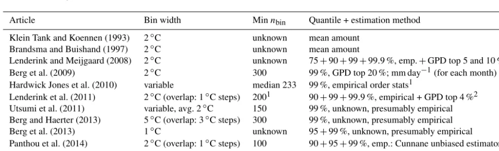
Table 1.P–T analysis methods used in the cited literature.
Article Bin width Minnbin Quantile + estimation method
Klein Tank and Koennen (1993) 2◦C unknown mean amount
Brandsma and Buishand (1997) 2◦C unknown mean amount
Lenderink and Meijgaard (2008) 2◦C unknown 75+90+99+99.9 %, emp.+GPD top 5 and 10 %
Berg et al. (2009) 2◦C 300 99 %, GPD top 20 %; mm day−1(for each month)
Hardwick Jones et al. (2010) variable median 233 99 %, empirical order stats1
Lenderink et al. (2011) 2◦C (overlap: 1◦C steps) 2001 90+99+99.9 %, empirical + GPD top 4 %2
Utsumi et al. (2011) variable, avg. 2◦C 150 99 %, unknown, presumably empirical
Berg and Haerter (2013) 5◦C (overlap: 3◦C steps) 300 99 %, unknown, presumably empirical
Berg et al. (2013) 1◦C unknown 95+99 %, unknown, presumably empirical
Panthou et al. (2014) 2◦C (overlap: 1◦C steps) 100 90+95+99 %, emp.: Cunnane unbiased estimator1
Westra et al. (2014) – – as in Lenderink et al. (2011)
1Personal communication per email.2As in climexp.knmi.nl (p).
2 Data and methods 2.1 Climate data
We analyzed publicly available time series of precipitation, temperature, and relative humidity from 142 stations across Germany from the German Weather Service (DWD, 2016). The stations are selected based on the length of available hourly time series. All selected datasets contain at least 15 years of observations, mostly 20 years. The R code for data selection, download, and analysis is available at https: //github.com/brry/prectemp.
To analyze only the nonzero precipitation records that are actually of interest for this article, values below 0.5 mm h−1 are omitted. This cutoff is in line with the cited literature and
is suitable because measurements of very low rainfall inten-sities have a high relative uncertainty. The values are then logarithmized to enable a comparison of rates of precipita-tion change across temperatures. Because of the very skewed nature of rainfall values, this also allows for better distribu-tion fits.
2.2 Temperature binning
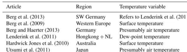
for-Table 2.Regions and temperatures used in the literature cited in Fig 1.
Article Region Temperature variable
Berg et al. (2013) SW Germany Refers to Lenderink et al. (2011)
Berg et al. (2009) Western Europe Surface temperature
Berg and Haerter (2013) Germany Presumably air temperature
Lenderink et al. (2011) Hongkong+NL Dew-point temperature
Hardwick Jones et al. (2010) Australia Surface temperature
Utsumi et al. (2011) Japan Presumably air temperature
mula based on observed relative humidity and air tempera-ture at 2 m height (see Buck, 1981).
Following the analysis method of Lenderink and Meij-gaard (2008) and Berg and Haerter (2013), we partition the hourly precipitation depths according to the event dew-point temperature. We use moving temperature bins with a fixed width of 2 K. Bin midpoints increase in 0.1◦steps.
2.3 Empirical quantiles
Empirical quantiles are estimated by a monotonic mapping of the ordered sample to sample-size-specific probabilities called plotting positions. This can be done in a variety of ways as reviewed by Hyndman and Fan (1996). Common to all is the fact that the portion to the right of the sample max-imum is left unresolved (no extrapolations) and receives the same probability as the maximum. Quantiles representing re-turn periods larger than the sample length are consequently mapped to that maximum. They are therefore underestimated – a fact apparently too trivial to have warranted any publica-tion. The empirical quantiles used in this article are computed based on the kn−+1/31/3 plotting positions (n=sample size,k= 1,...,n; see Hyndman and Fan, 1996).
2.4 Parametric quantiles
The parametric quantile estimates are obtained in a peak-over-threshold approach, where the generalized Pareto dis-tribution is fitted to the top 10 % of the sample. Quantiles are calculated from the fitted GPD.
We use the method ofLmoments to fit the GPD param-eters. They are analogous to the conventional statistical mo-ments (mean, variance, skewness, and kurtosis) but “robust [and] suitable for analysis of rare events of non-normal data.
L moments are consistent and often have smaller sampling variances than maximum likelihood in small to moderate sample sizes. L moments are especially useful in the con-text of quantile functions” (Asquith, 2016, 2011; Hosking, 1990).
To obtain the quantile from the fitted distribution, the given probabilities must be scaled with the conditional probability of the truncation. For example, if the 99 % quantile (Q0.99) is to be computed from the top 10 % of the data, Q0.90 of the truncated sample must be used. We refer to Q0.99 as the
“censored 99 % quantile”. Because five values are required to obtainLmoments, the minimum sample size at 90 % trunca-tion is 50 (45 values are discarded).
Selecting a suitable fitting method is of great importance in the context of sample size bias. For example, unlike moment-based procedures, maximum likelihood estimation (MLE) can still show an underestimation bias at small sample sizes, as shown in the Supplement. This happens in small samples (n <200) for distributions with bounded parameters (and the optimum of the likelihood function lying on the boundary). We refer to the Supplement for a comparison of the different methods.
The GPD quantile computation formula used in the source code of lmomco is
x(F )=
(
ξ+α
κ(1−(1−F )κ) ifκ6=0
ξ−α×log(1−F ) ifκ=0,
withξ =location, α=scale, κ=shape.
2.5 Sample size dependency
In Sect. 2.3, we pointed out that empirical methods inher-ently underestimate high quantiles in small samples. In order to quantify the potential effect in the context ofP–T rela-tionships, we set up the following experiment: to investigate the dependency of both quantile estimation methods on sam-ple size, we draw random samsam-ples from a defined popula-tion. This should optimally be a large set of values following a distribution observed in nature. We therefore use a pooled dataset with all the precipitation values observed at any of the 142 stations. From this population, we draw random samples of several sizes and compute empirical and parametric quan-tiles from each sample. For each sample size, this is done 1000 times, resulting in a corresponding quantile distribution depending on sample size.
2.6 SyntheticP–T relationship
tem-perature scaling over all temtem-perature ranges. The CC-scaling rate is constant, and the increase in high rainfall quantiles per degree Kelvin remains the same over all temperatures. When sampling from such synthetic data, any drop in theP–
T relationship must be a statistical artifact. For this purpose, we define a “temperature-dependent GPD” with parameters that depend on temperature. To achieve a realistic tempera-ture scaling, we base the parameters on the linear regression of the fitted parameters at several dew-point temperatures.
From that synthetic GPD, 1000 random samples are gen-erated for each temperature bin. The sample size corresponds to the average number of precipitation observations at the cli-mate stations in each bin. From these sets of random samples, the empirical and parametric 99.9 % quantiles are calculated.
3 Results
3.1 Sample size dependency
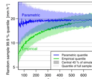
The dependence on sample size, as revealed by 1000 random draws per sample size from the pooled precipitation data, is shown in Fig. 2. The 99.9 % quantile of this population (n=1.16 million) is 19.5 mm h−1. It is strongly and consis-tently underestimated by the empirical estimator with shrink-ing sample size. For a sample size of 50, the median estimate is only 7 mm h−1. Realistic estimates are obtained only for samples larger than about 700, around which the estimates converge to the (true) population value. The parametric esti-mators do not exhibit this bias – only their variance increases with smaller samples (the uncertainty range is wider). This is a typical example of the well-known bias–variance tradeoff in estimation theory.
3.2 P–T relationship: empirical vs. parametric quantiles
The procedure of obtaining parametric (using the GPD) and empirical quantiles was applied per temperature bin to the datasets of each of the 142 stations. The empirical precipita-tion quantiles per bin are presented in the left panel of Fig. 3. The shape of theP–T relationships is consistent with the be-havior ofP–T relationships shown in Fig. 1 of the introduc-tory section. The empirical quantile estimates start decreas-ing between 15 and 20◦C. Some stations show the empiri-cal quantile drop more distinctly than others. The figure also shows the average across stations, where the drop becomes particularly clear. Compared to the red line depicting the CC scaling of 7 to 6 % K−1, the precipitation increase follows a
super-CC scaling with a rise that is steeper than the CC rate. This is in accordance with previous findings, e.g., by Berg and Haerter (2013).
The parametric estimates are displayed in the right panel. At temperature ranges where empirical quantiles decrease, parametric quantiles keep increasing. This difference is less pronounced for smaller quantiles (see Supplement Sect. S4).
100 200 300 400 500 600 700
Sample size n 5
10 20
Parametric quantile Empirical quantile Central 40% of simulations Quantile of full sample
Empirical Parametric
Random sample 99.9
% quantile [mm
h
-1]
Figure 2.Median of the empirical and parametric 99.9 % quantile
estimates depending on the size of samples drawn from all the pre-cipitation intensity values along with their uncertainty bands. The horizontal dashed line marks the empirical quantile of the complete
dataset (n=1.16 million). Forn >500, we used a step size of 10
(instead of 1) for the sample size, so the curve appears smoother there.
3.3 SyntheticP–T relationship
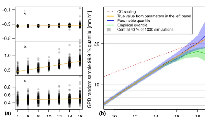
The syntheticP–T relationship that continuously rises with temperature (see Sect. 2.6) is defined with the parameters shown in the left panels of Fig. 4, where each dot repre-sents one of the stations. The right panel shows the median of the 99.9 % quantile estimates from random samples with the original sample sizes. Even though the distribution con-tinues to increase with temperature, empirical quantiles from random samples stagnate or drop around 18◦C where sample size decreases quickly. Parametric quantiles obtained by dis-tribution fitting do not drop and follow the theoretical quan-tile from the distribution function.
4 Discussion and conclusions
6 8 10 12 14 16 18 20
Dew-point temperature (mean of preceding 5 h) [°C]
Precipitation 99.9
% quantile [mm
h
-1]
5 10 20 50
100 (a)
Empirical
6 8 10 12 14 16 18 20
5 10 20 50
100 (b)
Parametric
Figure 3.The 99.9 % precipitation intensity per temperature bin with empirical and parametric quantile estimate (aandbrespectively). Each
line represents one of the 142 stations, with the black line as the average across stations. The red line denotes CC scaling as in Fig. 1. The
green line in(b)repeats the average from(a)for comparison.
−0.5 −0.3
−0.1 ξ
0.5 1.0
α
0.4 0.6 0.8
κ
4 6 8 10 12 14 16
Dew-point temperature bin midpoint [°C]
10 12 14 16 18
GPD random sample 99.9
% quantile [mm
h
-1]
10 20
CC scaling
True value from parameters in the left panel Parametric quantile
Empirical quantile
Central 40% of 1000 simulations
(a) (b)
Figure 4. (a)Parameters of a temperature-dependent GPD:ξ(location),α(scale), andκ(shape). The orange lines show a linear regression
as per Sect. 2.6.(b)Corresponding 99.9 % distribution quantile (orange) and median of the 99.9 % quantile estimates generated from samples
in 1000 random draws along with their variance bands.
size, and we verified this behavior in a set of Monte Carlo experiments. It turned out that the underestimation of high quantiles, such as those relevant for the upper portion of the CC-scaling relationship, can be substantial. We have shown that when empirical estimators are appropriately replaced by parametric ones, the high-temperature drop in CC scal-ing disappears. The method of parametric estimation is cru-cial, nevertheless, as similar small-sample biases are known, e.g., from using MLE estimators (see above and more exam-ples in the Supplement). The most robust estimates were ob-tained from moment-based methods. Past CC-scaling studies
that have relied on empirical or ML-based quantile estima-tors are likely affected by the small-sample artifacts for high temperatures that we have described here. For those, we find it necessary to revisit the corresponding estimation step us-ing other, e.g., moment-based, procedures. This may be es-pecially interesting for quantiles beyond the 99.9 % level.
rela-tionship is caused by a lack of moisture supply. It should be noted, though, that the use of dew-point temperatures only accounts for moisture that is already stored in the local at-mosphere. It does not account for large-scale moisture con-vergence which becomes more important with longer pre-cipitation duration intervals. This is evidence that the drop in empirical quantile estimates is precipitation independent; it is less a physical phenomenon but rather a statistical ar-tifact caused by small samples, and it can largely be over-come by employing parametric estimators. Still, alternative physical explanations considering physical processes should not lightly be discarded. Some were summarized briefly in Sect. 1. It might also, for example, be hypothesized that near-surface temperature is not an adequate proxy for air tempera-ture at the height where precipitation-forming patterns unfold on very warm days.
Parametric quantiles from fitted distributions provide a means to retrieve less biased estimates of extreme quan-tiles. The price to be paid is the larger uncertainty of those estimates. This should be quantified by confidence inter-vals or application to several datasets to avoid singular non-representative results. The parametric method requires sig-nificantly fewer data points in a sample than empirical quan-tiles need to converge to the actual (unknown) value. In the combination of small sample sizes and very high quantiles, the use of parametric quantiles is recommended.
Code and data availability. The datasets are freely available through the DWD Climate Data Center. The complete analysis code and more graphical results are available at https://doi.org/10.5281/ zenodo.892004.
The Supplement related to this article is available online at https://doi.org/10.5194/nhess-17-1623-2017-supplement.
Author contributions. BB conducted the analysis and wrote the manuscript. GB and MH came up with the original idea and pro-vided guidance and review.
Competing interests. The authors declare that they have no conflict of interest.
Acknowledgements. We wish to thank DWD for preparing and providing the datasets as well as William Asquith for reviewing our manuscript before submission. We are indebted to the reviewers for their many suggestions that led to the published version of this article.
Edited by: Uwe Ulbrich
Reviewed by: Reik Donner and two anonymous referees
References
Asquith, W. H.: Distributional analysis with L-moment statistics using the R environment for statistical computing, CreateSpace Independent Publishing Platform, http://scholar.google.com/ scholar?cluster=4144393830145643403&hl=en&oi=scholarr (last access: 15 September 2017), 2011.
Asquith, W. H.: lmomco: L-moments, Censored L-moments, Trimmed L-moments, L-comoments, and Many Distribu-tions, https://cran.r-project.org/package=lmomco (last access: 15 September 2017), 2016.
Berg, P. and Haerter, J. O.: Unexpected increase in pre-cipitation intensity with temperature. A result of
mix-ing of precipitation types?, Atmos. Res., 119, 56–61,
https://doi.org/10.1016/j.atmosres.2011.05.012, 2013.
Berg, P., Haerter, J. O., Thejll, P., Piani, C., Hagemann, S., and Christensen, J. H.: Seasonal characteristics of the relationship between daily precipitation intensity and sur-face temperature, J. Geophys. Res.-Atmos., 114, D18102, https://doi.org/10.1029/2009JD012008, 2009.
Berg, P., Moseley, C., and Haerter, J. O.: Strong increase in con-vective precipitation in response to higher temperatures, Nat. Geosci., 6, 181–185, https://doi.org/10.1038/ngeo1731, 2013. Brandsma, T. and Buishand, T. A.: Statistical linkage of daily
pre-cipitation in Switzerland to atmospheric circulation and temper-ature, J. Hydrol., 198, 98–123, https://doi.org/10.1016/S0022-1694(96)03326-4, 1997.
Buck, A. L.: New Equations for Computing Vapor
Pressure and Enhancement Factor, J. Appl.
Mete-orol., 20, 1527–1532,
https://doi.org/10.1175/1520-0450(1981)020<1527:NEFCVP>2.0.CO;2, 1981.
DWD: hourly precipitation records, ftp://ftp-cdc.dwd.de/pub/CDC/ observations_germany/climate/hourly/precipitation/historical/ (last access: 15 September 2017), 2016.
Haerter, J. O. and Berg, P.: Unexpected rise in extreme precipita-tion caused by a shift in rain type?, Nat. Geosci. 2, 372–373, https://doi.org/10.1038/ngeo523, 2009.
Hardwick Jones, R., Westra, S., and Sharma, A.: Observed relation-ships between extreme sub-daily precipitation, surface temper-ature, and relative humidity, Geophys. Res. Lett., 37, L22805, https://doi.org/10.1029/2010GL045081, 2010.
Hosking, J. R. M.: L-Moments: Analysis and Estimation of Distri-butions Using Linear Combinations of Order Statistics, J. Roy. Stat. B, 52, 105–124, 1990.
Hyndman, R. J. and Fan, Y.: Sample Quantiles in
Sta-tistical Packages, The American Statistician, 50, 361,
https://doi.org/10.2307/2684934, 1996.
Klein Tank, A. M. G. and Koennen, G. P.: The dependence of daily precipitation on temperature, Proceedings of the 18th annual cli-mate diagnostics workshop, Boulder, Colorado, 207–211, 1993. Lenderink, G. and Meijgaard, E. v.: Increase in hourly precipitation
extremes beyond expectations from temperature, Nat. Geosci. 1, 511–514, https://doi.org/10.1038/ngeo262, 2008.
Lenderink, G., Mok, H. Y., Lee, T. C., and van Oldenborgh, G. J.: Scaling and trends of hourly precipitation extremes in two dif-ferent climate zones – Hong Kong and the Netherlands, Hydrol. Earth Syst. Sci., 15, 3033–3041, https://doi.org/10.5194/hess-15-3033-2011, 2011.
Multi-Time-Scale and Event-Based Analysis, J. Hydrometeorol., 15, 1999–2011, https://doi.org/10.1175/JHM-D-14-0020.1, 2014.
Utsumi, N., Seto, S., Kanae, S., Maeda, E. E., and
Oki, T.: Does higher surface temperature intensify
ex-treme precipitation?, Geophys. Res. Lett., 38, L16708,
https://doi.org/10.1029/2011GL048426, 2011.