Application of RBFN for forward kinematics
solution of a parallel manipulator
Dr. Sudipto Chaki Associate professor,
Automobile Engineering department, MCKV Institute of Engineering
_____________________________________________________________________________________________________ Abstract - In the present work different architectures of Radial Basis Function Networks (RBFN) with supervised learning are trained and tested for solving forward kinematics (FK) of a 3-3 UPU manipulator which can predict end effector location uniquely for real time implementation of the manipulator. Performances of the architectures during training and simulation are also analysed in detail and its superiority over traditional backpropagation is also established. An attempt is also taken to find empirical equations to predict the error during training and simulation with variation in spread and fixed hidden layer neurons in RBFN for the present problem. Performance of the network for tracking a trajectory in a plane is also shown. Ultimately it is found that, the best architecture among tested can predict any arbitrary location in the workspace of the manipulator with maximum errors and average errors of 0.018339 cm and 0.001860 cm during simulation. As errors during simulation are confined only within a very small range it can be easily applied in real time applications.
Index Terms - Forward kinematics (FK), 3-3 UPU Manipulator, Radial Basis Function Networks (RBFN)
_____________________________________________________________________________________________________
I. INTRODUCTION
Generally the parallel manipulator consists of a moving platform attached with base plate by means of a set of identical parallel kinematic chains, called legs. The legs are usually equal to the degrees of freedom of the manipulator. Gradually it was found that parallel manipulators with lesser degrees freedom have certain advantages over conventional six limb parallel manipulators such as easier FK, larger work space, no need of complicated spherical joint etc. Initially manipulators having lesser degree of freedom are developed by Clavel [1] and Sernheim [2] known as 4-dof high-speed Delta Robot. Gradually Tsai and Joshi [3] have developed a 3 DOF UPU manipulator and its kinematics is analyzed. Kinematic analysis of such manipulators is performed in two phases. In the inverse kinematics (IK) solution of this manipulator, location of the centre of the moving platform is given as input to find out the length of the legs uniquely for the specific location of the manipulator. But generally solution of FK involves multiple possible location of the mobile platform for a known set of input leg length with respect to base frame and creates difficulty for real time application. For real time application it is required to determine a particular solution (the actual one) out of all possible solutions as fast as possible. As closed form solutions are found unable to find out an unique solution for end effector location, different numerical approaches were applied to conventional 6 DOF manipulators [4, 5, 6, 7,8,9,10,11]. But they were also found unsuitable for the real time implementation due to their inherent problem of large iteration time and tendency to reach local minima. Gradually neural network is found as a suitable supplement of the above methods for 6-6 manipulators in real time application [12,13,14]. In the present work neural network approaches are applied for forward kinematic analysis of a 3 DOF UPU manipulator developed by Tsai and Joshi [3]. Previously no attempt has been observed for solution of FK of this manipulator using neural networks.
In the present paper different architectures of RBFN are trained and tested for solution of the forward kinematics. Empirical equations are established to predict the error during training and simulation with variation in spread and fixed hidden layer neurons in RBFN for the present problem. Moreover, the performance of the best architecture among tested, is discussed in detail and its performance compared with traditional BP.
II. CONSTRUCTION OFTHEMANIPULATOR
In the present study a three degree of freedom parallel manipulator is considered where both the moving and base platform is of the shape of irregular triangle. Both the moving and base platforms are coupled by means of three legs. Ai and Bi are the vertices of moving platform and base plate respectively with respect to OUVW and OXYZ system. O and Oi are the centre of base and moving plate respectively.AiandBiare the position vectors of the vertices of the base plate with respect to origin of OUVWandOXYZcoordinate systems respectively.Liare length vectors of legs.In the present manipulator the base and the mobile platforms are similar that is they are of the same shape but of different sizes such that,
Ai= μBi( i = 1, 2 and 3) (1)
where μ is a given constant calledscaling factor.
So, Ai’s can be easily determined if Position vector Bi with respect to origin O in OXYZ coordinate is known for a specific value of μ. Each of the leg vectors are denoted fromBitoAibyLi, such that,
i i
i
A
B
L
iL
, i=1, 2 and 3 (2)Figure1. A 3-3 UPU Manipulator III. FORWARDKINEMATICSSOLUTION
Generation of dataset
In the present study O is the centre of the base plate known to be a fixed point (0, 0, 0) andBiis calculated.
is taken as0.5. The primary location O1 is assumed to be at (0, 0, 15) with respect to base platform. The upper platform is moved in different locations randomly within the workspace and positions of the O1 at every position are noted. Then IK is used here as a means of calculation of leg lengths.IfPbe the position vector between two origin points O and O1, the length of the each leg
can be obtained by
RE B P
RE B P
T i
i i
L2 (
) (
) i = 1,2,3. (3)Where E is 3x3 identity matrix and due to the specific structural constraint of the present manipulator rotation matrix, R is also taken as identity matrix.
ie.
( RE)B P
( RE)B P
12i T
i i
L i=1,2,3. (4)
Here, negative results are meaningless, so it can be omitted.This formulation is used here to find out the IK in the present problem only after getting the required information about
,R,BiandP.Set of leg lengths are calculated uniquely from (4).The feasible solution set generated in this way ultimately contains 2543 sets of position with corresponding set of the length of the legs. As all the data has been generated randomly in the workspace, it can be considered that they are free from bias. So, out of the total data set first 2500 set are considered as training data and rest 43 data set are as testing or simulation data. Here each set contains three input data such as leg lengths and three output data ie. position of the end effectors.
Training and simulation using artificial neural networks
One main advantage of artificial neural networks is their ability to model complex nonlinear relationships between multiple input variables and the required outputs. Generalization along with approximation is considered here as most important property of the feed forward ANN [15]. Generally they are massively parallel adaptive networks consists of simple nonlinear computing elements called neurons. Each neuron receives signals as input which passes through a weighted pathway in order to generate a linear weighted aggregation of the impinging signals. It can be then certainly transformed through an activation function to generate the output signal of the neuron. The activation functions may be binary threshold, linear threshold, Sigmoidal, Gaussian etc.
In the present problem numbers of input nodes are three representing the leg lengths from L1 to L3 respectively.
Consequently, number of nodes in the output layer is also three which represents the position coordinates of the end effector in X, Y and Z direction respectively. Number of neurons in the hidden layer can be varied according to the requirement.
Application of RBFN
A feed forward network RBFN is employed for the present problem where no weighted connection exists between input and hidden layer. It computes hidden neuron activations using Gaussian basis function which is an exponential of the Euclidean distance measure between the input vector and a prototype vector that characterizes the signal function at hidden neuron. It can be given by,
22
2
exp
X
X
(5)
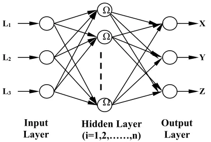
L1
L3 L2
Z Y X
Output Layer Input
Layer Hidden Layer(i=1,2,……,n) Ω Ω
Ω
Figure2. Architecture of the Radial Basis Function Networks Table 1. Training and Simulation Data for RBFN
In the present study RBFN is used for a function approximation problem where input and output variables has fixed three numbers of nodes and supervised learning is used here for training where the centre and output layer weights are updated after each epoch and network is considered to be trained only when the output error falls below a predetermined value. Altogether 16 different networks have been tested with spread factor varying from 0.5 to 2.0 with a constant basis function in order to find out the network with optimum approximation capability. Here all data in the input and output are normalized first and then fed as input and output to the networks. Mean square error (mse) is considered as criterion of performance of network during training and simulation. Before starting training, random initialization is used for weights. Each network is trained over 1000 epochs in this purpose. Then the trained network is simulated for the 43 sets of unknown test data. All the performance indices such as mean square error (mse), sum of the square error (sse) and mean average error (mae) are calculated for each case. The simulation is also done with the training or input data to show performance of the network with known value. All the training and simulation is done by MATLAB 7.0 in a Pentium 4, 3 GHz, and 512 MB PC. Training and simulation data for all the networks with RBFN are shown in the Table1.
Performance study of networks during training and simulation
In this section variation of number of neurons with sse during training is plotted in Fig.3. It is observed that the upto RBF 9 errors reduces rapidly with increase in number of spread but it after that reduction rate becomes very slow. Using Curve Fitting Toolbox of MATLAB 7.0 it is also observed that variation in spread can be fitted well with sse upto an R-square value of 0.9905. The curve can be expressed with an empirical equation at 95% confidence interval:
Network name
Training Simulation
Spread elapsedTime in sec SSE
With Unknown test data Trajectory
MSE SSE MAE MSE SSE MAE
(6)
Similarly from the curve plotted between spread and training time in Fig.4, it is observed that as spread increases, train time is also decreases exponentially with spread:
)
03586
.
0
exp(
28
.
34
)
174
.
3
exp(
55
.
65
)
(
x
x
x
f
(7)
Fitness of the curve at 95% confidence level is given by the R 2value of 0.9701. Fig.5 shows the change in mse during
simulation with respect to spread for different architectures. Here also nature of the plot remains same ie. exponential with the following equation:
)
-0.2084
exp(
010
-6.927e
)
-0.3328
exp(
007
-1.266e
)
(
x
x
x
f
(8) Efficiency of fit is given by R2value 0.9247.
Now from the equation of the curve as given in (6) and (8) variation of mse with spread during training and simulation can be directly calculated. Similarly, corresponding training time with increase in spread can also be directly obtained from (7). Thus, to know the effect of mse in training and simulation with any further increase in the spread, no more training is required for this specified problem. It can be directly predicted from (6), (7) and (8). Thus, for analyzing this specified problem using neural network with RBFN, requirement of training and simulation is ended here.
It is observed from Table 1 it is clear that within the tested range of RBFN, the network with 1.8 spread and 25 hidden layer neurons (RBF14) shows maximum reduction in sse upto 0.0036 during training and mse even upto 6.5385e-8 during simulation with test data which is different from training data. As RBF14 produces minimum mse during training the RBF with 1.8 spread and 25 hidden layer neurons is considered here as best architecture among tested and analyzed further.
Figure.3. Variation of sse With Spread During RBF Training
Figure.5. Variation of mse With Spread During Simulation Comparison with RBF14 and BP Performance study of networks during training and simulation
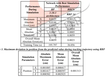
Here performance of the selected network RBF14 is compared with BP of 3-10-3 architecture during simulation to predict position of 43 arbitrary locations of the end effector within the workspace, which is different from training data. During this simulation, error in position is obtained from the difference between predicted positions with the actual one. While comparing error to predict position of all 43 arbitrary points within the workspace it is found that disregarding some large errors, variation of errors in RBF14 are confined in very small region compared to BP. Though it is referred to as large errors, from Table 2 it can be observed that, for BP the absolute maximum error in predicting position is confined only within 0.0365cm and which is further reduced to 0.0207 cm with the RBF14. Moreover, from Table 2 it is observed that the overall mean absolute error in predicting position with for RBF14 is only 0.0023cm, in comparison to 0.0059cm for BP. Naturally RBF14 not only shows significant reduction in maximum error but also truncates the mean absolute error in a great extent, in comparison to BP with 3-10-3 network. In addition to that, it is observed from Table3 that, training time of the BP is 195.797 s which are almost 6 times larger than training time of RBF6 that requires 36.056 s. Thus, RBF6 can be implemented online more effectively in comparison with 3-10-3 network due to much lesser training time requirement and greater error reduction capability during simulation to predict arbitrary position within workspace along with orientation of the end effector.
Table 2. Performance comparison of different architectures during simulation
Table 3. Maximum deviation in position from the predicted value during tracking trajectory using RBF14
Simulation Parameters
Absolute Maximum
Error (cm)
Mean Absolute
Error (cm)
Overall Mean Absolute
Error (cm) 1
Position X 0.001085 0.000417 0.001313
2 Y 0.001417 0.000597
3 Z 0.008502 0.002925
Performance of RBFN in tracking a trajectory
Though in the earlier section generalization capability of RBF 14 in predicting any arbitrary point within the workspace is already established, the present study is carried out to find out the capability of the manipulator to track an arbitrarily taken near circular trajectory in a plane at a height of 10 cm from the base as shown in Fig.6. RBF14 is further employed for the purpose. It is observed from Table. 3 that maximum absolute error in tracking the trajectory is 0.0085 cm only and overall mean absolute error is confined only within 0.0013 cm.
Performance During Simulation
Network with Best Simulation Performance
BP RBFN
3-10-3
architecture RBF 14 Maximum
Absolute Error (cm)
X 0.0121 0.0012
Y 0.0146 0.0204
Z 0.0365 0.02068
Mean Absolute Error(cm)
X 0.0029 0.0004
Y 0.0047 0.0005
Z 0.0100 0.0059
Overall Mean
Figure 6. Performance of RBF14 in Tracking Trajectory IV. CONCLUSION
In this paper, FK of a 3-3 UPU parallel manipulator is studied using neural networks in order to avoid limitations of the conventional closed form solution and numerical methods in real time application. Different architectures of RBFN are used for training and simulation. Different empirical equations are developed to directly predict the variation of mean square error (mse) during training and simulation and training time with number of hidden layer neurons without any further training. Ultimately during simulation, RBF network with 25 neurons and 1.0 spread are considered to be most efficient for the present problem due to its greater accuracy to predict any arbitrary point within the workspace. In comparison with BP having single hidden layer, RBFN has shown its superiority not only in accuracy to predict any unknown point within the workspace but also in training time, which is almost 6 times lesser than BP. Further RBFN is employed for tracking an arbitrary trajectory with overall mean absolute error of 0.0013 cm. There are no comparable literatures found to show such accuracy in simulation with unknown test value using RBFN for forward kinematics problem. But the accuracy shown by the best RBF network here in predicting an unknown point in the workspace is quite adequate for the moderate precision robot, although it may be yet behind the required accuracy in a very precise robotic application.
REFERENCE
[1] R. Clavel , 1988, ‘‘DELTA, A Fast Robot With Parallel Geometry,’’ 18th International symposium on Industrial Robots, pp. 91–100.
[2] F. Sternheim, 1987, ‘‘Computation of the Direct and Inverse Kinematic Model of the Delta 4 Parallel Robot,’’ Robotersysteme, 3, pp. 199–203.
[3] L.W.Tsai, and S. Joshi, 2000, ‘‘Kinematics and Optimization of a Spatial 3-UPU Parallel Manipulator,’’ ASME J. Mech. Des., 122 (4), pp. 439–446.
[4] J.P. Merlet ,2006, "Parallel robots”, Springer Science & Business Media, Vol. 128 .
[5] K.Cleary, T. Brooks, “Kinematic Analysis of A Novel 6-DOF Parallel,” Manipulator.IEEE Trans.on Robotics and Aut., 1993
[6] B.Dasgupta. T.S. Mruthyunjaya, “A Canonical Formulation of the Direct Position Kinematics Problem for a General 6-6 Stewart Platform,”Mechanism and Machine Theory, Vol. 29(6), 1994, pp.819-827
[7] C.W. Wampler, “Forward displacement analysis of general six-in-parallel SPS (Stewart) platform manipulators using SOMA coordinates,”Mechanism and. Machine.Theory, vol.31 (3), 1996, pp.331-337
[8] P.J. Parikh, and S.S.Lam, , 2009, "Solving the forward kinematics problem in parallel manipulators using an iterative artificial neural network strategy",The International Journal of Advanced Manufacturing Technology, Vol. 40, No. 5, 595-606
.[9] H. Singh, and N. Sukavanam,2013, "Stability analysis of robust adaptive hybrid position/force controller for robot manipulators using neural network with uncertainties",Neural Computing and Applications, Vol. 22, No. 7-8, 1745-1755
[10] M. Hosseini, and H. Daniali, "Weighted local conditioning index of a positioning and orienting parallel manipulator",Scientia Iranica, Vol. 18, No. 1, 115-120.
. [11] A.. Morell, M, Tarokh, and L. Acosta, 2013, "Solving the forward kinematics problem in parallel robots using support vector regression",Engineering Applications of Artificial Intelligence, Vol. 26, No. 7, (2013), 1698-1706.
[12]Z.Geng, L.Haynes, “Neural Network Solution For The Forward Kinematics Problem Of A Stewart Platform,”In Proc. Int. Conf. on Robotics and Automation, 1991,pp. 2650-2655
[13] M. Maleki, and R. Sahraeian, 2015, "Online monitoring and fault diagnosis of multivariate-attribute process mean using neural networks and discriminant analysis technique", International Journal of Engineering-Transactions B: Applications, Vol. 28, No. 11, 1634-1642.
[14]Choon seng Yee, Kah-bin Lim, 1997, “Forward kinematics solution of Stewart platform using neural networks,”
Neurocomputing, Vol. 16(4), pp.333-349
[15]K. Hornik, M. Tinchcombe . and H. White., 1989, “Multilayer feed forward networks are universal approximators,”