APPLICATION OF NUMERICAL OPTIMIZATION AS A TOOL FOR VALIDATION OF OPTIMIZED RESPONSE OF FLEXURAL STRENGTH OF WOOD ASH (HARDWOOD) PARTICLES REINFORCED POLYPROPYLENE WARPP

Sunday et al. World Journal of Engineering Research and Technology

APPLICATION OF NUMERICAL OPTIMIZATION AS A TOOL FOR

VALIDATION OF OPTIMIZED RESPONSE OF FLEXURAL

STRENGTH OF WOOD ASH (HARDWOOD) PARTICLES

REINFORCED POLYPROPYLENE WARPP

Aguh Patrick Sunday*1 and Ejikeme Ifeanyi Romanus2 1

Department of Industrial Production Engineering, Nnamdi Azikiwe University, Awka,

Anambra State, Nigeria.

2

Office of the Commissioner, Ministry of Environment, Beautification and Ecology, Awka,

Anambra State, Nigeria.

Article Received on 22/06/2017 Article Revised on 12/07/2017 Article Accepted on 02/08/2017

ABSTRACT

In this study, we investigated the adequacy of approximation of fitted

model to the real system. To meet this objective, the numerical

optimization method was applied as an alternative to the conventional

method by Suresh (2014) for the validation of optimized performance

characteristic (response) model. Box – Behnken design, a spherical

design, with all factorial and axial points at the same distance from the

center of the design was used to build a model for predicting and optimizing the flexural

strength of WARPP. The mathematical model equations (response surface models) were

derived from the response surface methodology (RSM) optimization process using Minitab

16 software. This response surface model is representable with nonlinear power equation and

second order polynomial of the four control factors. In the statistical analysis, the analysis of

variance (ANOVA) table, the coefficient of determination, R2 and the adjusted coefficient of determination, R2adj values and p values indicated that the model was adequate for

representing the experimental data. The p values show that the linear effects of volume

fraction (B), injection force (C), operating temperature (D) and quadratic effects of volume

fraction (B^2), injection force (C^2) and the interaction effects of volume fraction and

World Journal of Engineering Research and Technology

WJERT

www.wjert.org

*Corresponding Author

Aguh Patrick Sunday

Department of Industrial

Production Engineering,

Nnamdi Azikiwe

University, Awka, Anambra

injection force (B*C) and volume fraction and operating temperature (B*D) were highly

significant. To gain a better understanding of the control variables for optimal flexural

performance, the graphical models were presented as 3 – D response surface and 2 – D

contour graphs. The optimal setting for the particle size (A), volume fraction (B), injection

force (C) and operating temperature (D) were found to be 1.40mm, 5%, 200tons and 215oC respectively at the highest flexural strength value of 50.0933MPa. The predicted R2 value of 99.97% and adjusted R2 value of 99.99% are within 0.20 of each other indicating that the predicted response model and experimental data are in reasonable agreement (Mourabet et.

al., 2013).

KEYWORDS: Numerical optimization, Flexural strength, Box – Behnken design, Experimental design, Regression statistics and Validation.

INTRODUCTION

Wood ash particles reinforced polypropylene (WARPP) composite has been investigated to

determine its performance at optimal setting of parameters. The performance of WARPP is

effected by many factors such as wood ash particle size, volume fraction, injection force and

operating temperature of the injection moulding machine.

WARPP is a composite material that consist of polypropylene (PP) resin as the matrix

material and wood ash particles as the filler material. Wood ash engineering application has

been studied relatively by few researchers. Most of the applications had been to cement based

work. Abdullahi (2006) in his paper titled “characteristics of wood ash/OPC concrete”

reported that wood ash obtained from the combustion of wood can be related to fly ash since

fly ash is obtained from coal, a fossilized wood. Okunade (2008) in his research article titled

“the effect of wood ash and saw-dust admixture on the engineering properties of a burnt

laterite – clay brick” stated that wood ash admixture in line with its pozzolanic nature was

able to contribute in attaining denser products with higher compressive strength. Sanusi et.

al., (2013) investigated the influence of wood ash as an additive on the mechanical properties

of polymer matrix composite (fibre glass reinforced epoxy resin). The mechanical properties

investigated include tensile strength, impact and hardness strengths. Result of the research

revealed that addition of the wood ash into fibre glass reinforced epoxy resin composite

improved the tensile strength and impact strength up to 2.3% and 0.8% of wood ash addition

respectively. Hardness strength also increased progressively with the addition of wood ash.

studied the physical, chemical and microstructural properties of wood ash in order to

determine the potential applications for it. Goodman Mark Mendel (1998) conducted research

on the effects of wood ash additive on the structural properties of lime plaster. The objective

of the research was to determine the effects that wood ash imparted to lime plaster while

focusing upon the performance criteria relevant to base coat application such as water

retention, shrinkage, adhesion and permeability. However no application of wood ash was

made in thermoplastic polymer resin.

In this study, a research on the application of wood ash particles as potential filler materials

in polypropylene resin was conducted.

MATERIALS AND METHODS 1.1Material Selection

The materials used in this research are thermoplastic polymer, polypropylene (PP) resin as a

matrix material while wood ash particles were used as filler material. PP, a linear

hydrocarbon polymer was obtained from a resin chemical commercial outfit named POKEZ

chemicals at Onitsha while the wood ash (hardwood) was sourced locally. The wood ash was

obtained from 10Kg mass of saw dust that was burnt and allowed to smouldered in an open

space at ambient temperature for 12 hours. The characteristics (chemical compositions) of the

wood ash obtained from X- ray Fluorescence analysis is presented in Table 1.

1.2Chemical Modification of Wood Ash Particles Applied to Polypropylene.

Silane coupling agent was used as a chemical bonding agent in this work. The silane coupling

agent was in liquid form and has the name 3 – aminopropyltrimethoxy silane. The chemical

formula is





treated filler materials (wood ash particles) were added into the polypropylene resin in

volume fractions of 5%, 35% and 60% before injection moulding to produce the samples. To

investigate the bonding efficiency of the coupling agent, Fourier Transform Infrared

Spectroscopy (FTIR) test was performed so as to analyze the molecular vibrations of the

samples. The analyses were performed at Spring Board Chemical Research laboratory, Awka.

Different spectra produced from the analyses represented the “fingerprints” of the samples

with absorption peaks corresponding to the frequencies of vibrations of the bonds in the atom

of the materials. The absorbance intensities of the bonds were identified and recorded.

Absorbance intensity shows the influence of filler modification on light absorption of

materials. The sample with the smallest value of absorbance intensity signify the most porous

of all the samples. The spectra of three representative samples are presented and discussed in

chapter 4.

1.3Design of experiments.

Two experimental designs were applied in this work, namely Taguchi Robust Design (TRD)

and Response Surface Methodology (RSM). Taguchi experimental design method consists of

input variables that are divided into the following categories:

(i) Control factors: These are the design parameters of the product or process.

(ii) Noise (External) factors: These are factors whose values are difficult to control during

normal production process (Unal & Dean, 1991).

Taguchi techniques consider only the main effects of a model, and these are the first order

terms of the model. The limitations of Taguchi technique of not handling interaction effects

were handled by the application of RSM. RSM is a second order function for approximating

the response of factors with interaction effects. RSM model consists of first order and higher

order terms. In the application of RSM method, two special experimental designs considered

in fitting second order model to the response with minimum number of runs were:

(ii) Box – Behnken Design.

A CCD with 3 design variables at 2 levels has 23 factorial points, 2 x 3 axial points and 1 central point (Hill and Hunter, 1966). Box – Behnken design is a three level factors design

that are widely used in response surface methods to fit second order models to responses

(Relia, 2013). The advantages of Box – Behnken design include:

(i) The fact that it is a spherical design and requires factors to be run at only three levels.

That is all factorial and axial points are at the same distance from the center of the design.

(ii) There are no runs where all factors are at either +1 or -1 levels.

Figure 1(a): CCD for 3 design variables at 2 levels (b)Box - Behnken design for three factors at 3 levels.

1.4Fitting a Second Order Model to the Design Data.

The limitation of TRD method of not handling interaction effects and RSM to handle noise

effects was solved by extending the result of TRD with RSM.

The response function of a second order model is best characterized by multivariate power

equation. The data obtained from Taguchi robust design was linearized on the assumption

according to Chapra and Canale (2006) that the experimental result follow a power law

model of the form:

an a

a a

N C B A a

Y 1 2 3...

0

 (1)

And that the response surface is optimized by a second order polynomial equation expressed

as:

 

 

    









 

 

1 1 2 1

2 1

q

i q

j

j i ij q

i

i ii q

i i i

O X X X X

where Y is the predicted response used as a dependent variable,

q is the number of independent variables (factors),

Xi (i = 1, 2) is the input factors,

βo is the constant coefficient, and

βi, βij and βii are the coefficients of linear, interaction and quadratic terms respectively.

The coefficient parameters were estimated using regression as analysis tool for evaluating log

data of input parameters presented in Table 2, and expressed as a power law model of the

form of equation (2).

) 2755 . 0 ^ ( * ) 1053 . 0 ^ ( * ) 0463 . 0 ^ ( * ) 0002 . 0 ^ ( * 041676689 .

7 A B C D

Yflex   (3)

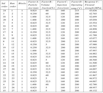
Twenty – seven observed responses presented in Table 2 were obtained by evaluating

equation (3) using the data values of the factors’ levels of Box – Behnken design matrix.

Table 2: Experimental design matrix of Box – Behnken design for optimization of power

function (equation) of flexural strength of PP composites.

The response surface models were stated as equations (9) and (10) for coded and uncoded

factors presented and discussed in chapter 4, section 4.2.

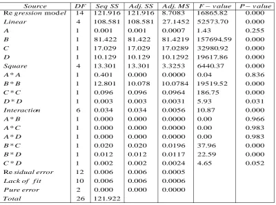
The test for statistical significance of the response model is presented in the analysis of

variance (ANOVA) Table 3, and also as Table 4 in chapter 4, section 4.3, where it was

discussed.

Table 3: Analysis of variance (ANOVA) for RSM optimization of WARPP for flexural strength. 052 . 0 000 . 0 000 . 0 983 . 0 983 . 0 966 . 0 000 . 0 031 . 0 000 . 0 000 . 0 836 . 0 000 . 0 000 . 0 000 . 0 000 . 0 255 . 0 000 . 0 000 . 0 65 . 4 59 . 22 96 . 37 00 . 0 00 . 0 00 . 0 87 . 10 93 . 5 75 . 186 52 . 19519 04 . 0 37 . 6440 86 . 19617 92 . 32980 59 . 157694 43 . 1 70 . 52573 82 . 16865 0000 . 0 0006 . 0 0005 . 0 0024 . 0 0117 . 0 0196 . 0 0000 . 0 0000 . 0 0000 . 0 0056 . 0 0031 . 0 0964 . 0 0784 . 10 0000 . 0 3253 . 3 1292 . 10 0289 . 17 4219 . 81 0007 . 0 1452 . 27 7083 . 8 000 . 0 006 . 0 006 . 0 002 . 0 012 . 0 020 . 0 000 . 0 000 . 0 000 . 0 034 . 0 003 . 0 096 . 0 078 . 10 000 . 0 301 . 13 129 . 10 029 . 17 422 . 81 001 . 0 581 . 108 916 . 121 922 . 121 000 . 0 006 . 0 006 . 0 002 . 0 012 . 0 020 . 0 000 . 0 000 . 0 000 . 0 034 . 0 003 . 0 096 . 0 801 . 12 401 . 0 301 . 13 129 . 10 029 . 17 422 . 81 001 . 0 581 . 108 916 . 121 26 2 10 12 1 1 1 1 1 1 6 1 1 1 1 4 1 1 1 1 4 14 Re * * * * * * * * * * mod Re . . Total error Pure f it of Lack error sidual D C D B C B D A C A B A n Interactio D D C C B B A A Square D C B A Linear el gression value P value F MS Adj SS Adj SS Seq DF

Source  

Where A, B, C and D are the particle size, volume fraction, injection force and operating

temperature respectively. The coefficients with the factors A, B, C and D represent the effects

of the factors, while the coefficients with A2, B2, C2, D2 and those with A*B, A*C, A*D, B*C, B*D and C*D represent the quadratic effect and interaction between the two factors

respectively.

determination (R2adj) modifies R2 by taking into account the number of predictors (terms) in the model. The R2adj. close to the R2 value insured a satisfactory adjustment of the quadratic model to the experimental data. The predicted R2 is a measure of how well the model predicted the response value. The R2adj. and R2pred. are within 0.20 of each other showing that they are in reasonable agreement (Mourabet et. al., 2013). The regression statistics can be

checked using a numerical method for coefficient of determination (R2), adjusted R2 (R2adj.) as expressed in equation (4) and (5) (Trinh and Kang, 2010).

residual el

residual SS SS

SS R

 



m od 2

1 (4) 2 .





1

1 R

p n

n

R adj 

  

 (5)

where SS is the sum of squares.

n is the number of experiments.

p is the number of predictors (terms) in the model, not counting the constant term.

3: Validation of the Model.

It is necessary to check the fitted model to ensure that it provides an adequate approximation

to the real system. Unless the model shows an adequate fit, proceeding with the optimization

of the fitted response surface is likely to give misleading result. The graphical optimization

method i.e. optimization plot was used as a primary tool for optimization. The graphical

technique was validated using numerical method. The crucial phase of numerical

optimization is the assignment of optimization parameters. There are three optimization

parameters namely maximum, minimum and target that define each desirability index, di. The

desirability function di is defined differently based on the objective of the response according

to Relia Wiki (2013) and is expressed as:

(i) If the response is to be maximized, di is defined as:

    

  

 

  

  



L

T

Y

di

0

1 Y T

T Y L

L Y

i i i

  



(6)

where T represents the target value of the ith response ( the highest value) and L represents the acceptable lower limit value for the response.

    

  



  

 

  

  





U Y

U Y T

T Y i

d

i i i

i

T

U

Y

U

1

0

(7)

Where U represents the acceptable upper limit of the response and T is the smallest value.

(iii)For a specific target response value, di is defined as:

  

   

 

  

 



      

 

      

 











U Y

U Y T

T Y L

L Y

i i

d

i i i i

i

T

U

Y

U

L

T

L

Y

0

0

(8)

By the evaluation of equation (6) for maximization as a desirability, using the maximum and

minimum values of Flexural strength in Table 2 at desirability index di = 1, Yi > T.

Which gives Yi 49.132

From the optimization plot of Figure 5 presented and discussed in chapter 4 section 4.4, Yi =

50.093MPa.

4 RESULTS AND DISCUSSIONS

4.1 Results of characterization of WARPP samples

The quality of WARPP samples used in this study was evaluated using microscopic method –

Fourier transform infrared spectroscopy (FTIR) technique. Three different spectra were

produced from three different samples. The spectra were represented by Figures 2, 3 and 4.

Their vertical axes represent the absorption peaks while the horizontal axes are the

wavenumbers.

Absorption

   

 

  

500 . 41 132 . 49

500 . 41

Figure 2: A plot of transmission against wave number of sample 1.

Sample 1: 0.25(5 % vol. fraction), from Figure 2 we have the following peaks.

3406.78- O-H stretch vibration (H bond)

2983.83 – C-H stretch vibration, (C-H) alkane group.

1749.52 – C=O stretch vibration

883.52 – C-H bend (deformation vibration).

Figure 3: A plot of Transmission vs. Wave number of sample 1.40(35 % vol. fraction).

For sample 2: 1.40(35 % vol. fraction), from Figure 3 the absorption peaks are:

3486.43 – O-H stretch vibration

3000.56 – C-H stretch vibration

1616.94 – C = O stretch vibration

Figure 4: A plot of Transmission vs. wave number of sample 3.

For sample 3: 0.80(60 % volume fraction), from Figure 4 the absorption peaks are:

3420.22 – O – H stretch vibration.

3024.21 – C-H stretch vibration.

1709.54 – C=O stretch vibration

828.50 – C-H bend (deformation vibration).

The identifiable mode of vibration by the chemical bonds are stretch vibration and

deformation vibration.

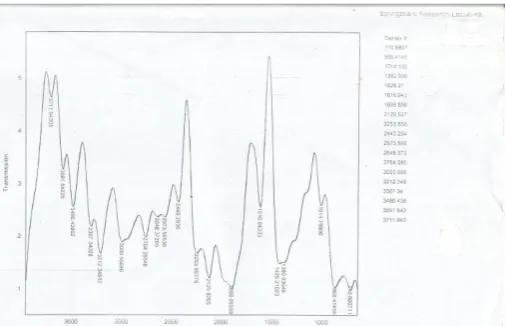
Discussion of the FTIR spectrum.

In Figure 2, the region of absorbance peaks is 3800.762cm-1 and 760.4085cm-1, for the sample composition designated as 0.25(5% vol. fraction). Figures 3 and 4 had their

absorbance peaks in the regions of 3711.943cm-1 and 710.881cm-1 for sample composition designated as 1.40(35% vol. fraction), and 3768.433cm-1 and 828.508cm-1 for the sample composition designated as 0.80(60% vol. fraction). The corresponding absorbance ranges are

3040.353cm-1, 3001.062cm-1 and 2939.9247cm-1 respectively. The corresponding absorbance intensity range is 26.667 – 10.000 = 16.667%, 46 – 10 = 36%, and 40 – 10 = 30%

respectively. Absorbance intensity indicates the influence of filler modification on light

absorption. The lowest absorbance intensity value signifies that composite of the designated

composition 0.25(5 % vol. fraction) may be more porous.

In Figure 2, where the intensity of absorption is 3406.78 cm-1 is showing strong hydrogen bonding with stretch vibration. The hydrogen bonding is due to de-methylation of the

methoxyl group (-OCH3) in silane coupling agent, which splited and CH3 being replaced by

signifies deformation vibration (bending) of C-H bond. The absorption band 1,749.52

signifies the carboxyl, c = o stretch vibration.

Similarly, the absorption peak in Figure 3 is around 3486.43cm-1. Also de-methylation of the methoxyl group in silane coupling agent occurred, and the methyl group was replaced by

hydrogen atom. The absorption band 3000.56cm-1 is due to C-H stretch vibration of the methoxyl group. The absorption band 868.41cm-1 signifies deformation vibration of C-H bond.

In Figure 4, the peak is around 3420.22cm-1 and is due to the hydrogen bonding (O-H) stretch vibration. De-methylation also took place with the methoxyl group in silane coupling agent

splited, creating condition for the production of hydrogen bond. The absorption band

868.41cm-1 is due to C-H deformation vibration.

4.2: Result of the evaluation and optimization of flexural strength of WARPP.

The response surface models are second order regression models that contain

15











parameters include the coefficients for main effects A, B, C and D, coefficients for quadratic

main effects A^2, B^2, C^2 and D^2 and the coefficients for two factor interaction effects

A*B, A*C, A*D, B*C, B*D and C*D and a constant value.

For coded factor,

2 ^ 1345 . 0 2 ^ 3747 . 1 2 ^ 0021 . 0 9188 . 0 1913 . 1 6048 . 2 0078 . 0 007 .

44 A B C D A B C

Y       

. * 0245 . 0 * 054 . 0 * 07 . 0 * 0003 . 0 * 0003 . 0 * 0005 . 0 2 ^ 024 .

0 D  A B A C A D B C B D C D



(9) For uncoded factor,

2 ^ 0063012 .

0 10154 . 0 0505655 .

0 176485 .

0 0175116 .

0 6945 .

25 A B C D A

Y     

C A E B

A E D

E C

E

B^2 8.40365 05 ^2 1.06481 04 ^2 3.16206 05 * 1.08696 05 *

00181774 .

0        



D C E D

B E C

B E D

A

E 05 * 6.36364 05 * 1.30909 04 * 4.08333 05 *

89855 .

2       



(10)

4.3: Test for statistical significance

052 . 0 000 . 0 000 . 0 983 . 0 983 . 0 966 . 0 000 . 0 031 . 0 000 . 0 000 . 0 836 . 0 000 . 0 000 . 0 000 . 0 000 . 0 255 . 0 000 . 0 000 . 0 65 . 4 59 . 22 96 . 37 00 . 0 00 . 0 00 . 0 87 . 10 93 . 5 75 . 186 52 . 19519 04 . 0 37 . 6440 86 . 19617 92 . 32980 59 . 157694 43 . 1 70 . 52573 82 . 16865 0000 . 0 0006 . 0 0005 . 0 0024 . 0 0117 . 0 0196 . 0 0000 . 0 0000 . 0 0000 . 0 0056 . 0 0031 . 0 0964 . 0 0784 . 10 0000 . 0 3253 . 3 1292 . 10 0289 . 17 4219 . 81 0007 . 0 1452 . 27 7083 . 8 000 . 0 006 . 0 006 . 0 002 . 0 012 . 0 020 . 0 000 . 0 000 . 0 000 . 0 034 . 0 003 . 0 096 . 0 078 . 10 000 . 0 301 . 13 129 . 10 029 . 17 422 . 81 001 . 0 581 . 108 916 . 121 922 . 121 000 . 0 006 . 0 006 . 0 002 . 0 012 . 0 020 . 0 000 . 0 000 . 0 000 . 0 034 . 0 003 . 0 096 . 0 801 . 12 401 . 0 301 . 13 129 . 10 029 . 17 422 . 81 001 . 0 581 . 108 916 . 121 26 2 10 12 1 1 1 1 1 1 6 1 1 1 1 4 1 1 1 1 4 14 Re * * * * * * * * * * mod Re . . Total error Pure f it of Lack error sidual D C D B C B D A C A B A n Interactio D D C C B B A A Square D C B A Linear el gression v alue P v alue F MS Adj SS Adj SS Seq DF

Source  

As can be seen from ANOVA Tables 4, the F - values obtained for the significant terms are

greater than the F – value of 2.64 at 95% significance (F0.95, 14, 12) of a standard F- distribution

table. This confirmed the adequacy of the model fit. The significance of each term in the

models was indicated by the p – values associated with the terms. A term is not significant if

p – value is greater than 0.05. The value 0.05 indicates the significance level of observed

effects. Significance level is the probability of the observed significant effect being due to

pure error. That is, the risk of saying that a factor is significant when in fact it is not.

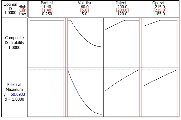
4.4 Optimization Plot.

Optimization plot is the graphical representation of the dependent and independent variables

at their optimal settings. The optimal values of the factors were indicated in the plot. The

optimization plot indicated a maximum predicted value of 50.0933MPa flexural strength with

particle size of 1.40mm, volume fraction of 5%, injection force of 200tons and operating

Cur

High Low 1.0000D Optimal

d = 1.0000 MaximumFlexural

y = 50.0933

1.0000 Desirability Composite

185.0 215.0 120.0

200.0 5.0

60.0 0.250

1.40 Vol. fra Inject. Operat.

Part. si

[1.40] [5.0] [200.0] [215.0]

Figure 5: Optimization plot for flexural strength.

CONCLUSIONS

This work has demonstrated the application of Numerical optimization in validating the

optimized performance characteristics of flexural strength of WARPP. From the study carried

out, the following conclusions were drawn:

1. The result of statistical analysis (ANOVA) shows that the control and interaction factors

B, C, D and B*B, C*C, B*C and B*D have significant effects on the flexural strength of

WARPP.

2. The flexural strength of WARPP is in the range of 46.65MPa – 50.09MPa.

3. The response model of WARPP is representable with nonlinear power law and second

order polynomial equation.

4. The optimal value of flexural strength of WARPP was obtained with the particle size of

1.40mm, volume fraction of 5%, injection force of 200tons and operating temperature of

215oC.

5. The results of the optimization plot were obtained at a condition (desirability = 1) that

satisfied each of the parameters without compromising on any of them (i.e. they are

equally weighted). This demonstrated that to obtain a maximum amount of information in

a short period of time, with the least number of experiments, RSM and optimization plot

can be successfully applied for modeling and optimizing the flexural strength of WARPP.

6. The flexural strength of WARPP obtained from the validation of the model is in the range

was appropriate for validating the optimized performance characteristics of flexural

strength of WARPP.

REFERENCES

1. Abdullahi M. Characteristics of Wood Ash/OPC Concrete. Leonardo Electronic Journal

of Practices and Technologies, 2006; (8): 9-16.

2. Chapra S. C., and Canale R. P. Numerical Methods for Engineers. 5th Edition, McGraw-Hill, New York, 2006; 460 – 462 and 623 – 625.

3. Goodman M. M. The effects of wood ash additive on the structural properties of line,

1998. plaster. [Online]. Available: http://archive.org/stream/effects of

woodashoogood/effectsofwoodash.

4. Hill W. J and Hunter W. G. A review of response surface methodology: A literature

survey, 1966. Technometrics, 571- 591. Mead, R. and D. J. Pike… [Online]. Available:

www.stat.rudgers.edu/home/buyske/591/Lect06.pdf

5. Mourabet M., El Rhilassi A., El Boujaady H., Bennani-Ziatni M., Taitai A. Use of

Response Surface Methodology for Optimization of Fluoride adsorption in an aqueous

Solution by Brushite. Arabian Journal of Chemistry, 2013; 12: 028.

6. Naik Tarun R., Kraus Rudolph, and Kumar R. Wood Ash: A new source of Pozzolanic

material. Report No. CBU Centre for by-product utilization. University of Wisconsin,

2001.

7. Okunade E. A. The Effect of Wood Ash and Sawdust Admixtures on the Engineering

Properties of a Burnt Latrite-Clay. Journal of Applied Sciences, 2008; 8: 1042-1048.

8. Radharamanan R. and Ansui A. P. Quality Improvement of a Production Process using

Taguchi Methods. Proceedings of Institute of Industrial Engineers’ Annual Conference,

Dallas, Texas, 2001.

9. Relia Wiki: Response Surface Methods for Optimization. [Online].

http://reliawiki-org/index.php/Response_Surface_methods_for_opti.. (Accessed Sept. 19), 2013.

10. Sanusi O. M., Oyinlola A. K., Akindapo J. O. Influence of Wood Ash on the Mechanical

properties of Polymer Matrix Composite Developed from Fibre glass and Epoxy resin.

International Journal of Engineering Research and Technology (IJERT). ISSN 2278 –

0181, 2013; 2(12).

11. Suresh R. K. Multi Objective Optimization during Turning of AISI 8620 Alloy Steel

using Desirability Function Analysis. International Journal of Engineering Science &

12. Trinh T. K. and Kang L. S. Application of Response Surface Method as an Experimental

Design to Optimize Coagulation Tests. Journal of Environmental Engineering Research,

2010; 15(2): 63 – 70.

13. Unal R. & Dean B. Taguchi Approach to Design Optimization for Quality and Cost: An

Overview. Presented at the Annual Conference of the International Society of Parametric

Analysis, 1991.