Linear Neurons and Their Learning Algorithms

ISSN: 2334-2366 (Print), 2334-2374 (Online) Copyright © The Author(s). All Rights Reserved. Published by American Research Institute for Policy Development DOI: 10.15640/jcsit.v6n2a1 URL: https://doi.org/10.15640/jcsit.v6n2a1

Linear Neurons and Their Learning Algorithms

Ying Liu

1

Abstract

In this paper, we introduce the concepts of Linear neurons, and new learning algorithms based on Linear neurons, with an explanation of the reasons behind these algorithms. First, we briefly review the Boltzmann Machine and the fact that the invariant distributions of the Boltzmann Machine generate Markov chains. We then review the θ-transformation and its completeness, i.e. any function can be expanded by θ-transformation. We further review ABM (Attrasoft Boltzmann Machine). The invariant distribution of the ABM is a θ-transformation; therefore, an ABM can simulate any distribution. We then discuss that the ABM algorithm is only the first algorithm in a family of new algorithms based on the θ-transformation. We introduce the simplest algorithm in this family based on Linear neurons. We also discuss the advantages of this algorithm: accuracy, stability, and low time complexity.

Keywords: AI, Boltzmann machine, Markov chain, invariant distribution, Completeness, Deep Neural Network.

1. Introduction

Neural networks and deep learning currently provide the best solutions to many supervised learning problems. In 2006, a publication by Hinton, Osindero, and Teh [1] introduced the idea of a “deep” neural network, which first trains a simple supervised model; then adds on a new layer on top and trains the parameters for the new layer alone. You keep adding layers and training layers in this fashion until you have a deep network. Later, this condition of training one layer at a time is removed.

After Hinton‟s initial attempt of training one layer at a time, Deep Neural Networks train all layers together. Examples include Tensor Flow [30], Torch [31], and Theano [32]. Google‟s Tensor Flow is an open-source software library for dataflow programming across a range of tasks. It is a symbolic math library, and also used for machine learning applications such as neural networks.[6] It is used for both research and production at Google. Torch is an open source machine learning library and a scientific computing framework. Theano is a numerical computation library for Python. The approach using the single training of multiple layers gives advantages to the neural network over other learning algorithms.

One question is the existence of a solution for a given problem. This will often be followed by an effective solution development, i.e. an algorithm for a solution. This will often be followed by the stability of the algorithm. This will often be followed by an efficiency study of solutions. Although these theoretical approaches are not necessary for the empirical development of practical algorithms, the theoretical studies do advance the understanding of the problems. The theoretical studies will prompt new and better algorithm development of practical problems. Along the direction of solution existence, Hornik, Stinchcombe, & White [33] have shown that the multilayer feedforward networks with enough hidden layers are universal approximators. Roux & Bengio [34] have shown the same, Restricted Boltzmann machines are universal approximators of discrete distributions.

Hornik, Stinchcombe, & White [33] establish that the standard multilayer feedforward networks with hidden layers using arbitrary squashing functions are capable of approximating any measurable function from one finite dimensional space to another to any desired degree of accuracy, provided sufficiently many hidden units are available. In this sense, multilayer feed forward networks are a class of universal approximators. Deep Belief Networks (DBN) are generative neural network models with many layers of hidden explanatory factors, recently introduced by Hinton, Osindero, and Teh, along with a greedy layer-wise unsupervised learning algorithm. The building block of a DBN is a probabilistic model called a Restricted Boltzmann machine (RBM), used to represent one layer of the model. Restricted Boltzmann machines are interesting because inference is easy in them and because they have been successfully used as building blocks for training deeper models. Roux & Bengio [34] proved that adding hidden units yield a strictly improved modeling power, and RBMs are universal approximators of discrete distributions.

In our earlier paper [15], we provide yet another proof. The advantage of this proof is that it will lead to multiple new learning algorithms. In our approach, Deep Neural Networks implement an expansion and this expansion is complete. In this paper, we will present a new algorithm based our earlier paper [15]. In addition to neural network algorithms, there are numerous learning algorithms. We select a few such algorithms below.

Principal Component Analysis [16-17] is a statistical procedure that uses an orthogonal transformation to convert a set of vectors into a set of values of linearly uncorrelated variables called principal components. The number of principal components is less than or equal to the number of original variables.

Sparse coding [18-19] minimizes the objective: L sc =||WH−X|| 22 + λ || H|| 1

Where, W is a matrix of transformation, H is a matrix of inputs, and X is a matrix of the outputs. λ implements a trade of between sparsity and reconstruction.

Auto encoders [20-25] minimizes the objective: L ae =||W σ (WTX) – X || 22

Where σ is some neural network functions. Note that L sc looks almost like L ae once we set H=σ(W T X) . The difference is that 1) auto encoders do not encourage sparsity in their general form; 2) an auto encoder uses a model for finding the codes, while sparse coding does so by means of optimization.

K-means clustering [26-29] is a method of vector quantization which is popular for cluster analysis in data mining. K-means clustering aims to partition n observations into k clusters. Each observation belongs to the cluster with the nearest mean, serving as a prototype of the cluster. This results in a partitioning of the data space into k clusters.

If we limit the learning architecture to one layer, all of these algorithms have some advantages for some applications. The deep learning architectures currently provide the best solutions to many supervised learning problems; in other words, two layers are better than one layer. In 2006, a publication by Hinton, Osindero, and Teh[1] introduced the idea of a “deep” neural network, which first trains a simple supervised model; then adds on a new layer on top and trains the parameters for the new layer alone. In this approach of completing one layer before moving into the next layer, one can argue that each layer can be any learning algorithm and the neural network is one of many candidates in each layer.

The advantage of Deep Neural Network is to train all layers together; for example, TensorFlow [30], Torch [31], and Theano [32]. Google‟s TensorFlow is an open-source software library for dataflow programming across a range of tasks. It is a symbolic math library, and also used for machine learning applications such as neural networks.[3] It is used for both research and production at Google. Torch is an open source machine learning library and a scientific computing framework. Theano is a numerical computation library for Python. The approach with single training of multiple layers gives advantages to the neural network over other learning algorithms.

This approach advances the current state of understanding of neural networks by stating that neural network is a part of a larger and complete expansion, where completeness means any function can be expanded. Based on the above discussion regarding the importance of the neural network, this different perception matters; it has both practical and theoretical significance. An alternative to the direction of “deep”, higher order is another direction. These two directions are equivalent [15]. In addition, both deep and higher order can be combined. In this paper, we review θ-transformation and will introduce a new family of learning algorithms characterized by θ-θ-transformation.

In section 2, we briefly review how to use probability distributions in a Supervised Learning Problem. In this approach, given an input A, an output B, and a mapping from A to B, one can convert this problem to a probability distribution [4-8] of (A, B): p ( a, b ) , a ϵA, b ϵ B. If an input is a ϵA and an output is b ϵ B, then the probability p (a, b) will be close to 1. One can find a Markov chain [9] such that the equilibrium distribution of this Markov chain, p (a, b), realizes, as faithfully as possible, the given supervised training set.

In section 3, the Boltzmann machines [4-8] are briefly reviewed. Our discussion concentrates on the distribution space of the Boltzmann machine rather than the neural aspects. All possible distributions together form a distribution space. All of the distributions, implemented by Boltzmann machines, define a Boltzmann Distribution Space, which is a subset of the distribution space [11-14]. Given an unknown function, one can find a Boltzmann machine such that the equilibrium distribution of this Boltzmann machine realizes, as faithfully as possible, the unknown function. A natural question is whether such an approximation is possible. The answer is that this approximation is not yet a good approximation.

In section 4, we review the ABM (Attrasoft Boltzmann Machine) [10] which has an invariant distribution. An ABM is defined by two features: (1) an ABM with n neurons has neural connections up to the nth _{order; and (2) all of the} connections up to nth _{order are determined by the ABM algorithm [10]. By adding more terms in the invariant distribution} compared to the second order Boltzmann Machine, ABM is significantly more powerful to simulate an unknown function. Unlike the Boltzmann Machine, ABM‟s emphasize higher order connections rather than lower order connections. The Boltzmann Machine and the ABM are at the opposite end of the neuron orders.

In section 5, we review θ-transformation [11-14].

In section 6, we review the completeness of the θ-transformation [11-14]. The θ-transformation is complete; i.e. given a function, one can find a θ-transformation by converting it from the x-coordinate system to the θ-coordinate system.

In section 7, we discuss how the invariant distribution of an ABM implements a θ-transformation [11-14], i.e. given an unknown function, one can find an ABM such that the equilibrium distribution of this ABM realizes precisely the unknown function. Therefore, an ABM is complete.

In section 8, we show that the ABM algorithm is derived from the θ-transformation. We call the neurons in the ABM algorithm the exponential neurons, because of its exponential generating function. We introduce a new algorithm, and we will call the neurons in the new algorithm, linear neurons, because of its generating functions. The new algorithm uses summation in expansion, while the ABM algorithm uses multiplication in expansion. Therefore, the new algorithm is more stable.

In section 9, we introduce a simple example to test the algorithm.

2. Basic Approach

The basic supervised learning [2] problem is: given a training set {A, B}, where A = {a1, a2, … } and B = {b1, b2, …}, find a mapping from A to B. It turns out that if we can reduce this from a discrete problem to a continuous problem, it is very helpful. The first step is to convert this problem to a probability [4-8]:

p = p (a, b), a ϵ A, b ϵ B.

If a1 matches with b1, the probability is 1 or close to 1. If a1 does not match with b1, the probability is 0 or close to 0. This can reduce the problem of inferencing a mapping from A to B to inferencing a distribution function. An irreducible finite Markov chain possesses a stationary distribution [9].

3. Boltzmann Machine

A Boltzmann machine [4-8] is a stochastic neural network in which each neuron has a certain probability to be 1. The probability of a neuron to be 1 is determined by the Boltzmann distribution. The collection of the neuron states: x = ( x1, x2, ..., xn )of a Boltzmann machine is called a configuration. The configuration transition is mathematically described by a Markov chain with 2n _{configurations x ϵ X, where X is the set of all points, ( x1, x2, ..., xn ). When all of the} configurations are connected, it forms a Markov chain. A Markov chain has an invariant distribution [9]. Whatever initial configuration that a Boltzmann starts from, the probability distribution converges over time to the invariant distribution, p(x). The configuration x ε X appears with a relative frequency of p(x) over a long period of time.

A Boltzmann machine [4-8] defines a Markov chain. Each configuration of a Boltzmann machine is a state of the Markov chain. A Boltzmann machine has a stable distribution. Let T be the parameter space of a family of Boltzmann machines. An unknown function can be considered as a stable distribution of a Boltzmann machine. Given an unknown distribution, a Boltzmann machine can be inferred such that its invariant distribution realizes, as faithfully as possible, the given function. Therefore, an unknown function is transformed into a specification of a Boltzmann machine.

More formally, let F be the set of all functions. Let T be the parameter space of a family of Boltzmann machines. Given an unknown f ε F, one can find a Boltzmann machine such that the equilibrium distribution of this Boltzmann machine realizes, as faithfully as possible, the unknown function [4-8]. Therefore, the unknown, f, is encoded into a specification of a Boltzmann machine, t ϵ T. We call the mapping from F to T as a Boltzmann Machine Transformation: F  T [11-14].

Let T be the parameter space of a family of Boltzmann machines, and let FT be the set of all functions that can be inferred by the Boltzmann Machines over T; obviously, FT is a subset of F. It turns out that FT is significantly smaller than F so it is not a good approximation for F. The main contribution of the Boltzmann Machine is to establish a framework for inferencing a mapping from A to B.

4. Attrasoft Boltzmann Machines (Abm)

The invariant distribution of a Boltzmann machine [4-8] is:

If the threshold vector does not vanish, the distributions is:

By rearranging the above distribution, we have: e

=

p(x) c-Tixi+i<jMijxixj

It turns out that the third order Boltzmann machines have the following type of distributions:

An ABM [11-14] is an extension of the higher order Boltzmann Machine to the maximum order. An ABM with n neurons has neural connections up to the nth _{order. All of the connections up to the n}th _{order are determined by the ABM} algorithm [10]. By adding additional higher order terms to the invariant distribution, ABM is significantly more powerful to simulate an unknown function.

By adding additional terms, the invariant distribution for an ABM is: e

= p(x) H_,

.

x

...

x

x

+

...

+

x

x

x

+

x

x

+

x

+

=

H

n 2 1 12..n n i3

i2 i1 i1i2i3 3

i2 i1 i i 2 i

i 1

0 1 12

1

















e

b

=

p(x)

i<jMijxixj.

.

e b =

p(x) i<jMijxixj-Tixi

e =

ABM is significantly more powerful to simulate an unknown function. As more and more terms are added, from the second order terms to the nth _{order terms, the invariant distribution space will become larger and larger. Like} Boltzmann Machines in the last section, ABM implements a transformation, FB T. We will show that this ABM transformation is complete so that given any function f ϵ F, we can find an ABM, t ϵ T, such that the equilibrium distribution of this ABM realizes precisely the unknown function.

5. Θ - Transformation 5.1 Basic Notations

We first introduce some notations used in this paper [11-14]. There are two different types of coordinate systems: the x-coordinate system and the θ-coordinate system [11-14]. Each of these two coordinate systems has two representations, x-representation and θ-representation. An N-dimensional vector, p, is:

)

p

...

,

p

,

p

(

=

p

_{0 1 N-1} ,

which is the x-representation of p in the x-coordinate systems.In the x-coordinate system, there are two representations of a vector:

{ pi } in the x-representation, and

{ pmi1i2 ..im } in the θ-representation.

In the θ-coordinate system, there are two representations of a vector:

{ θi } in the x-representation, and

{ θmi1i2 ..im } in the θ-representation.

The reason for the two different representations is that the x-representation is natural for the x-coordinate system, and the θ-representation is natural for the θ-coordinate system.

The transformations between { pi } and { pmi1i2 ..im} , and those between { θi } and { θmi1i2 ..im}, are similar. Because of this similarity, only the transformation between {pi} and {pmi1i2 ..im} will be introduced. Let N = 2n be the number of neurons. An N-dimensional vector, p, is:

Consider px , because x ϵ { 0, 1, ... N - 1 = 2n - 1 } is the position inside a distribution, then x can be rewritten in the binary form:

Some of the coefficients, xi , might be zero. In dropping those coefficients which are zero, we write:

This generates the following transformation:

where

In this θ-representation, a vector p looks like:

).

p

...

,

p

,

p

(

=

p

_{0 1 N-1}

.

2

x

+

2

x

+

...

+

2

x

=

x

0

1 1 2 1

-n n

. 2 + 2 + ... + 2 = ...x x x =

x i -1 i-1 i-1

im i2 i1

1 2 m

p

=

p

=

p

i_mi ...i _{x 2}im-1_{+...+ 2}i2-1₊₂i1-1 m

2 1

_ ,

n. i < ... < i < i

p

p

p

p

p

p

,

p

,

p

₀ 1_{1 1}2

,

₁3

,...,

12₂

,

13₂

,

₂23

,

...,

₃123

,...}

{

The 0-th order term is

p

₀, the first order terms are:

p

₁1

,

p

2₁

,

p

₁3

,...

, … The first few terms in the transformation between { pi } and { pmi1i2 ..im} are:

The x-representation is the normal representation, and the θ-representation is a form of binary representation.

Example Let n = 3, N = 2n _{= 8, and consider an invariant distribution:} { p0, p1, p2, p3, p4, p5, p6, p7},

where p0 is the probability of state x = 0, … . There are 8 probabilities for 8 different states, x = {0, 1, 2, …, 7}. In the new representation, it looks like:

p

p

p

p

p

p

,

p

,

p

1233

23 2 13 2 12 2 3 1 2 1 1 1

0

,

,

,

,

,

}.

{

Note that the relative positions of each probability are changed. The first vector, { p0, p1, p2, p3, p4, p5, p6, p7}, is in the x-representation and the second vector

{

p

₀

,

p

1₁

,

p

₁2

,

p

₁3

,

p

12₂

,

p

₂13

,

p

₂23

,

p

₃123} is in the θ-representation. These two representations are two different expressions of the same vector.

5.2 θ-Transformation

Denote a distribution by p, which has a x-representation in the x-coordinate system, p(x), and a θ-representation in the θ-coordinate system, p(θ). When a distribution function, p(x) is transformed from one coordinate system to another, the vectors in both coordinates represent the same abstract vector. When a vector q is transformed from the x-representation q(x) to the θ-x-representation q(θ), and then q(θ) is transformed back to q'(x), then these two vectors are equal: q'(x) = q(x). The θ-transformation uses a function F, called a generating function. The function F is required to have the inverse:

. F = G I, = GF =

FG -1

Let p be a vector in the x-coordinate system. As already discussed above, it can be written either as:

)

p

...

,

p

,

p

(

=

p(x)

_{0 1 N-1} , Or

)

p

,

...

,

p

;

p

,

...

,

p

;

p

...,

,

p

;

p

(

=

p(x)

_{0 1}1 ₁n 12_{2 2}n-1,n 123₃ 12..n_n .

The θ-transformation transforms a vector from the x-coordinate to the θ-coordinate via a generating function. The components of the vector p in the x-coordinate, p(x), can be converted into components of a vector p(θ) in the θ-coordinate:

...

,

p

=

p

p

=

p

,

p

=

p

,

p

=

p

,

p

=

p

,

p

=

p

p

=

p

,

p

=

p

,

p

=

p

8 4 1 7 123 3 6 23 2

5 13 2 4 3 1 3 12 2

2 2 1 1 1 1 0

), , ... , ; , ... , ; ..., , ; ( = ) p( 12..n n 123 3 n 1, -n 2 12 2 n 1 1 1

0

















Or ). ... , , ( = )

p(





0



1



N-1

Let F be a generating function, which transforms the x-representation of p in the x-coordinate to a θ-representation of p in the θ-coordinate system. The θ-components are determined by the vector F[p(x)] as follows:

Where n. i < ... < i < i

1 1 2 m

Prior to the transformation, p(x) is the x-representation of p in the x-coordinate; after transformation, F[p(x)] is a θ-representation of p in the θ-coordinate system.

There are N components in the x-coordinate and N components in the θ-coordinate. By introducing a new notation X:

then the vector can be written as:

By using the assumption GF = I, we have: }

X G{ =

p(x) 



J J ,

where J denotes the index in either of the two representations in the θ-coordinate system.

The transformation of a vector p from the x-representation, p(x), in the x-coordinate system to a θ-representation, p(θ), in the θ-coordinate system, is called θ-transformation [11-14].

The θ-transformation is determined by [11-14]:

x

...

x

x

+

...

+

x

x

x

+

x

x

+

x

+

=

F[p(x)]

n 2 1 12..n n i3 i2 i1 i1i2i3 3 i2 i1 i i 2 i i 1

0 1 12

1

















... x x x x = X = X x x x = X = X , x x = X = X , x x = X = X , x = X = X , x x = X = X x = X = X , x = X = X , = X = X 4 3 2 1 8 4 1 3 2 1 7 123 3 3 2 6 23 2 3 1 5 13 2 3 4 3 1 2 1 3 12 2 2 2 2 1 1 1 1 1 0 0 , 1 X =

F[p(x)] 



J J.

The inverse of the θ-transformation [11-14] is:

5.3 An Example

Let an ANN have 3 neurons:

( x1, x2, x3 ) and let a distribution be:

{ p0, p1, p2, p3, p4, p5, p6, p7}. Assume that the generating functions are: F(y) = log (y), G(y) = exp ( y ).

By θ-transformation, the components are [11-14]:

p

p

=

p

p

=

p

=

0 2 2 0 1 1 0

1

log

,



log

,



log



,

p

p

p

p

=

p

p

p

p

=

p

p

=

p

p

p

p

=

2 0 6 6 1 0 5 5 0 4 1 0 4 4 4 2 3

3

log

,



log

,



log

,



log



,

The inverse are:

), exp( ), exp( ), exp( , )

exp( 0 1 0 1 2 0 2 3 0 1 2 3

0 



p 







p 







p 















p ), exp( ), exp( ),

exp( 0 4 5 0 1 4 5 6 0 2 4 6

4 







p 















p 















p

).

exp( 0 1 2 3 4 5 6 7

7 































p

Because of the nature of the exponential function, the 0 probability is 0 = e -∞_{, so the minimum of the probability, pi , will} be some very small value, ε, rather than 0 to avoid singularity.

Example

Let p = {2, 7, 3, 8, 2, 5, 5, 6}, then θ = {0.693, 1.252, 0.405, -0.271, 0, -0.336, 0.510, -0.462}. Example

Let θ = {0, 0, 0, 0, 0, 0, 0, 2.302}, then p = {1, 1, 1, 1, 1, 1, 1, 10}. Example

Let θ = {2.302, -0.223, -1.609, 1.832, -0.510, -0.875, 1.763, -1.581}, then p = {10, 8, 2, 10, 6, 2, 7, 3 }.

6. Θ – Transformation Is Complete

Because the θ-transformation is implemented by a normal function, FG = GF = I, as long as there is no singular points in the transformation, any distribution function can be expanded. For example, in the last section, we require pi >= ε, which is a predefined small number.

7. Abm Is Complete

An ABM with n neurons has neural connections up to the nth _{order. The invariant distribution is:} e

= p(x) H_,

).

+

...

+

+

...

+

+

+

+

...

+

+

+

G(

=

p

i ... i i m i i 2 i i 2 i i 2 i 1 i 1 i 1 0 i ... i i m m 2 1 m 1 -m 3 1 2 1 m 2 1 m 2 1

















p

p

p

p

p

p

p

p

=

p

p

p

p

p

p

p

p

=

=

0 6 5 3 4 2 1 7 0 23 2 13 2 12 2 3 1 2 1 1 1 123 3 123 3

7



log

log

.

x

...

x

x

+

...

+

x

x

x

+

x

x

+

x

+

=

H

n 2 1 12..n n i3 i2 i1 i1i2i3 3 i2 i1 i i 2 i i 1

0 1 ₁ 12

















An ABM implements a θ-transformation [11-14] with: F(y) = log (y), G(y) = exp ( y ).

Furthermore, the “connection matrix” element can be calculated as follows [11-14]:

The reverse problem is as follows: given an ABM, the invariant distribution can be calculated as follows [11-14]:

Therefore, an ABM can realize a θ-expansion, which in turn can approximate any distribution. ABM is complete [11-14]. Write the above equation:

).

...

...

...

(

=

p

i ... i i m i i 2 i i 2 i i 2 i 1 i 1 i 1 0 i ... i i m m 2 1 m 1 -m 3 1 2 1 2 2 1 m 2 1

















exp(

)

exp(

)

exp(

)

exp(

)

exp(

)

exp(

)

exp(

)

exp

We call the neurons in the ABM algorithm the exponential neurons, because of its exponential generating function. The ABM algorithm uses multiplication expansion, which raises the question of stability. Therefore, we expect to improve this algorithm.

8. A New Algoritm

If we can convert the multiplication expansion to addition expansion, then the performance will be more stable. Let :

G = X, F = X,

from section 5, we have:

...

p

p

...

p

p

p

...

p

p

=

i_mi...i i_m..._-2i i_m..._-2i _m..._{-4 m}i..._-1i _mi_-...₁i i_m..._-3i i ... i i m 3 -m 1 m 2 1 -m 1 m 3 2 -m 1 m 2 1 m 2

1



















.

+

...

+

+

...

+

+

+

+

...

+

+

+

=

p

i ... i i m i i 2 i i 2 i i 2 i 1 i 1 i 1 0 i ... i i m m 2 1 m 1 -m 3 1 2 1 m 2 1 m 2 1

















We call the neurons in the new algorithm as linear neurons, because of its generating functions. The new algorithm uses summation in expansion.

For simplicity, we will continue to call the cell “neurons”. Because G = F = I, we call these neurons identify neurons. Example: let an ANN have 3 neurons, ( x1, x2, x3 ) and let a distribution be:

{ p0, p1, p2, p3, p4, p5, p6, p7},

...

p

p

...

p

p

p

...

p

p

=

i ... i 3 -m i ... i 1 -m i ... i 1 -m ... 4 -m i ... i 2 -m i ... i 2 -m i ... i i m i ... i i

m _{1 m-1 2 m 1 m-3}

Then,

), (

), (

), (

, )

( 0 1 0 1 2 0 2 3 0 1 2 3

0 



p 







p 







p 















p

), (

), (

),

( 0 4 5 0 1 4 5 6 0 2 4 6

4 







p 















p 















p

).

( 0 1 2 3 4 5 6 7

7 































p

This is the starting point for the new algorithm. When the expansion is complete, it has the advantage of accuracy. When the expansion uses addition, it has the advantage of stability. As we will show below, it also has a third advantage of fast training (low time complexity).

The L1 –distance between two configurations is:

d ( x’, x ) =| x’1−x1| + | x’ 2−x2 | + … For example, d (111, 111) = 0; d (111, 110) = 1.

We now introduce a new algorithm, the Linear neuron learning algorithm, which can be summarized into a single formula:

)) , ( ( ^

2 D d xii...i x

m i

... i i

m12 m  12 m



, if d xii...i x D

m12 m 

 ( , )

0

0





ii...i

m12 m , if d x i x D ...

i i

m12 m, )

(

Where d(_xii...i ,x)

m12 m is the distance between a neuron configuration, x, and a training neuron configuration,

x

i ... i i m12 m, and D is called a connection radius. Beyond this radius, all connections are 0.

The linear neurons learning algorithm is: Step 1. The First Assignment (d=0)

The first step is to assign the first connection matrix element for training vector, x = xim1i2...im. We will assign: θx =



im1i2...im = 2D,

while D is the radius of the connection space. Step 2. The Rest of the Assignment

The next step is to assign the rest of the weight:

)) , ( ( ^

2 D d xii...i x

m i

... i i

m12 m  12 m



, if d xii...i x D

m12 m 

 ( , )

0

0





ii...i

m12 m , if d x x D i

... i i

m12 m, )

(

Step 3. Modification

The algorithm uses bit “1” to represent a pattern or a class; so, the input vectors or the output vectors cannot be all 0‟s; otherwise, these coefficients are 0.

Step 4. Retraining

Repeat the last three steps for all training patterns; if there is an overlap, take the maximum values:



ii...i

m12 m(t+1) = max {



i ... i i

m12 m (t),



i ... i i

m12 m }.

If we set D = 2, then the possible elements are: 2D-d _{= 4, 2, 1, and 0. There is one term for d = 0; there are no more} than n terms for d = 1; and there are no more than n(n-1)/2 terms for d = 2. Assume there are m training vectors, the time complexity for training is:

T = O (m n2_). In general, T = O (m nD_).

9. An Example

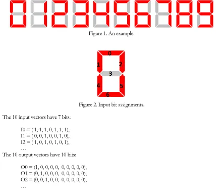
In this section, we will first use the linear neuron algorithm; then we will use the square and power neuron algorithms. The example is to identify simple digits in Figure 1 [1, 2, 13]. Each digit is converted into 7 bits: 0, 1, …, 6. Figure 2 shows the bit location.

Figure 1. An example.

Figure 2. Input bit assignments. The 10 input vectors have 7 bits:

I0 = ( 1, 1, 1, 0, 1, 1, 1), I1 = ( 0, 0, 1, 0, 0, 1, 0), I2 = ( 1, 0, 1, 0, 1, 0, 1), …

The 10 output vectors have 10 bits: O0 = (1, 0, 0, 0, 0, 0, 0, 0, 0, 0), O1 = (0, 1, 0, 0, 0, 0, 0, 0, 0, 0), O2 = (0, 0, 1, 0, 0, 0, 0, 0, 0, 0), …

The 10 training vectors have 17 bits:

T0 = (I0, O0) = ( ( 1, 1, 1, 0, 1, 1, 1), (1, 0, 0, 0, 0, 0, 0, 0, 0, 0) ), T1 = (I1, O1) = ( ( 0, 0, 1, 0, 0, 1, 0), (0, 1, 0, 0, 0, 0, 0, 0, 0, 0) ), …

We will set the radius: D = 2; the possible elements are: 2D-d _{= 4, 2, 1, and 0. We will work out a few examples. First, we} rewrite T1 as:

x

2593 = ( ( 0, 0, 1, 0, 0, 1, 0), (0, 1, 0, 0, 0, 0, 0, 0, 0, 0) ). The first connection element (0-distance) is: 259 4

3 



. There are two coefficients for d = 1: 29 2

2 59

2 







. T1 generates

3 coefficients. 25 0

2 



, due to step 3 of the algorithm; in this case, the output vector is all 0‟s. Next, we rewrite T7 as:

x14,2,5,14 = ( ( 1, 0, 1, 0, 0, 1, 0), (0, 0, 0, 0, 0, 0, 0, 1, 0, 0) ). The first connection element (0-distance) is: 1,2,5,14 4

4 



. There are 3 coefficients for d=1: 2,5,14 2

3 14 , 5 , 1 3 14 , 2 , 1

3 









There are 3 coefficients for d = 2: 5,14 1

2 14 , 2 2 14 , 1

2 











. T7 generates 7 coefficients.

Last, we rewrite T4 as:

x

15,2,3,5,11 = ( ( 0, 1, 1, 1, 0, 1, 0), (0, 0, 0, 0, 1, 0, 0, 0, 0, 0) ),

the first connection element (0-distance) is: 1,2,3,5,11

4

5





. There are 4 coefficients for d=1:

2

11 , 5 , 3 , 2 4 11 , 5 , 3 , 1 4 11 , 5 , 2 , 1 4 11 , 3 , 2 , 1

4 















. There are 6 coefficients for d = 2: 1,3,11 ... 1

2 11 , 2 , 1

3 



 



. T4 generates 11

coefficients.

After training the linear neuron algorithm with {T0, T1, …, T9}, all of the connection coefficients,



ii...i m12 m, are calculated. For example, the probability is

p

259₃ , if the input is „1‟ and the output is in class 1; the probability is

p

258₃ , if the input is „1‟ and the output is in class 0; the probability is

p

2₃,5,10, if the input is „1‟ and the output is in class 2; …

Section 7 provides the formula to calculate the probability of each (input, output) pair:

.

+

...

+

+

...

+

+

+

+

...

+

+

+

=

p

i ... i i m

i i 2 i

i 2 i i 2

i 1 i

1 i 1 0 i ... i i m

m 2 1

m 1 -m 3

1 2 1

m 2

1 m

2 1

















For example,

+

+

+

+

+

+

+

=

p



0



12



15



19



225



292



259



2593 259

3 .

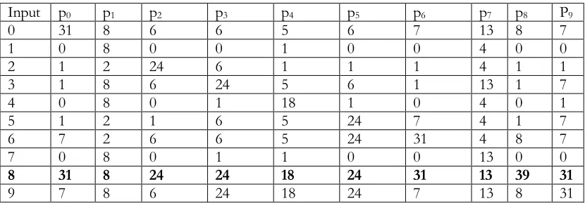
The character recognition results are given in Figure. 3, where the first column is input, then the next 10 columns are output. The output probability is not normalized in Figure 3. The relative probability for (input = 0, output = 0) is 31; those for (input = 0, output = 1) are 8; those for (input = 0, output = 2) are 6; … . So if the input is digit 0, the output is identified as 0. In this problem, the output is a single identification, so the largest weight determines the digit classification. In each case, all input digits are classified correctly.

Input p0 p1 p2 p3 p4 p5 p6 p7 p8 P9

0 31 8 6 6 5 6 7 13 8 7

1 0 8 0 0 1 0 0 4 0 0

2 1 2 24 6 1 1 1 4 1 1

3 1 8 6 24 5 6 1 13 1 7

4 0 8 0 1 18 1 0 4 0 1

5 1 2 1 6 5 24 7 4 1 7

6 7 2 6 6 5 24 31 4 8 7

7 0 8 0 1 1 0 0 13 0 0

8 31 8 24 24 18 24 31 13 39 31

9 7 8 6 24 18 24 7 13 8 31

Figure 3. The results from the new linear neuron algorithm without normalization

10. Conclusion

An ABM with n neurons has neural connections up to the nth _{order. We have observed that θ-transformation} defines a whole family of neurons. The θ-neurons generally emphasize higher order neurons rather than lower order neurons. The ABM uses exponential neurons. In this paper, we use linear neurons. We discussed that the ABM algorithm is only the first algorithm in a family of new algorithms based on the θ-transformation. We introduced the simplest algorithm in this family. We also discussed the advantages of this algorithm: accuracy, stability, and low time complexity.

Acknowledgements

I would like to thank Gina Porter for proof reading this paper.

Reference

Hinton, G. E., Osindero, S. and Teh, Y., “A fast learning algorithm for deep belief nets,” Neural Computation 18, pp 1527-1554.

Edgar Sanches-Sinencio and Clifford Lau, Editors, Artificial Neural Networks, IEEE Press, 1992. Ying Liu and Shaohui Wang, Completeness Problem of the Deep Neural Networks, submitted.

S. Amari, K. Kurata, and H Nagaoka, "Information geometry of Boltzmann machine," IEEE Trans., Neural Network, Vol. 3, No. 2, pp. 260 - 271.

Cihan H. Dagli, Editor, “Intelligent Engineering Systems Through Artificial Neural networks,” Vol. 5, ASME Press, pp. 757 - 850, 1995.

William Byrne, "Alternating Minimization and Boltzmann Machine Learning," IEEE Trans., Neural Network, Vol. 3, No. 4, pp. 612 - 620.

N. H. Anderson and D. M. Titterington, “ Beyonf the Binary Boltzmann Machine,” IEEE Trans., Neural Network, Vol. 6, No. 5, pp. 1229 - 1236.

C. T. Lin and C. S. G. Lee, “A Multi-Valued Boltzmann Machine,” IEEE Trans., SMC, Vol. 25, No. 4, pp. 660 - 668. W. Feller, An introduction to probability theory and its application, John Wiley and Sons, 1968.

Ying Liu, US Patent No. 7,773,800, http://www.google.com/patents/US7773800, Feb, 2002.

Ying Liu, "Image Compression Using Boltzmann machines," Proc. SPIE, Vol. 2032, pp. 103 - 117, July, 1993. Ying Liu, "Boltzmann Machine for Image Block Coding," Proc. SPIE. Vol. 2424, pp. 434 - 447, Feb., 1995.

Ying Liu, "Character and Image Recognition and Image Retrieval Using the Boltzmann Machine," pp. 706 - 715, Proc. SPIE. Vol. 3077, April 1997.

Ying Liu, "Two New Classes of Boltzmann Machines," Proc. SPIE, Vol. 1966, pp.162 - 175, April, 1993.

Liu, Y. and Wang, S. (2018) Completeness Problem of the Deep Neural Networks. American Journal of Computational Mathematics, 8, 184-196. doi: 10.4236/ajcm.2018.82014.

Jolliffe I.T. Principal Component Analysis, Series: Springer Series in Statistics, 2nd ed., Springer, NY, 2002, XXIX, 487 p. 28 illus. ISBN 978-0-387-95442-4.

H., & Williams, L.J. "Principal component analysis.". Wiley Interdisciplinary Reviews: Computational Statistics, 2: 433– 459, (2010).

Olshausen, Bruno A. "Emergence of simple-cell receptive field properties by learning a sparse code for natural images." Nature 381.6583 (1996): 607-609.

Gupta, N; Stopfer, M, "A temporal channel for information in sparse sensory coding.". Current Biology 24 (19): 2247–56 (October 2014)..

Bengio, Y. (2009). "Learning Deep Architectures for AI" (PDF). Foundations and Trends in Machine Learning 2. Modeling word perception using the Elman network, Liou, C.-Y., Huang, J.-C. and Yang, W.-C., Neurocomputing,

Volume 71, 3150–3157 (2008).

Autoencoder for Words, Liou, C.-Y., Cheng, C.-W., Liou, J.-W., and Liou, D.-R., Neurocomputing, Volume 139, 84–96 (2014).

David E. Rumelhart, Geoffrey E. Hinton, and Ronald J. Williams, "Learning internal representations by error propagation" (1986).

Bourlard, H.; Kamp, Y. (1988). "Auto-association by multilayer perceptrons and singular value decomposition". Biological Cybernetics 59 (4–5): 291–294.

MacQueen, J. B. (1967). Some Methods for classification and Analysis of Multivariate Observations. Proceedings of 5th Berkeley Symposium on Mathematical Statistics and Probability 1. University of California Press. pp. 281–297. Steinhaus, H. (1957). "Sur la division des corps matériels en parties". Bull. Acad. Polon. Sci. (in French) 4 (12): 801–804. A. B. Lloyd, S. P. (1957). "Least square quantization in PCM". Bell Telephone Laboratories Paper. Published in journal

much later: Lloyd., S. P. (1982). "Least squares quantization in PCM" (PDF). IEEE Transactions on Information Theory 28 (2): 129–137.

E.W. Forgy (1965). "Cluster analysis of multivariate data: efficiency versus interpretability of classifications". Biometrics 21: 768–769.

TensorFlow, https://www.tensorflow.org/. Torch, http://torch.ch/.

Theano, http://deeplearning.net/software/theano/introduction.html.

K. Hornik, M. Stinchcombe, and H. White (1989) Multilayer Feedforward Networks are Universal Approximators, Neural Networks, Vol. 2, pp. 359-366.