Forestry & Natural-Resource Sciences Last Correction: Apr. 10, 2013
MICRO-DETAIL COMPARATIVE FOREST SITE ANALYSIS
USING HIGH-RESOLUTION SATELLITE IMAGERY
Chris J Cieszewski, Roger C Lowe, Pete Bettinger, Arun Kumar
WSFNR, University of Georgia, Athens GA 30602 USA
Abstract. This study presents comparative analysis of high-resolution satellite imagery taken on different
dates around a detected incident of interest. Under an assumption of a micro-detail land monitoring and disturbance detection interests we compared the patterns of image captured disturbances on the analyzed site and leveraged their interpretation with knowledge published on relevant subjects. The incident of interest was the Polish Air Force One TU-154M plane destruction on April 10, 2010. We analyzed the image changes on a micro-detail level, tracked over time and considered with respect to the patterns of destruction and the plane debris size distribution in space, and compared these against information from the broader engineering literature describing destruction patterns of thin walled structures, such as planes and cars. Then, we compared the spatial distribution of the debris between the pictures taken on different dates. In this analysis, we also considered onground changes in soil moisture and landscape features between different images.
Keywords: Satellite images; land monitoring; thin walled structure crashing; image analysis; image correlation analysis.
1
Introduction
Modern forest management relies heavily on geo-graphic information systems (GIS) and remote sensing technology, particularly satellite imagery. Satellite im-agery is used extensively in forest inventory (Meng et al., 2009a, 2007a; Zawadzki et al., 2004a) and planning (Liu and Cieszewski, 2009; Liu et al., 2009; Zawadzki et al., 2005a,b), quantitative silviculture (Lowe et al., 2009; Meng and Cieszewski, 2006), as well as disturbance mon-itoring (Franke et al., 2012; Olsson et al., 2012), carbon tracking (Asner, 2009; Pelletier et al., 2012), vegetation monitoring (Alcaraz-Sequra et al., 2008), contemporary forest management (Meng et al., 2009b, 2007b; Zawadzki et al., 2004b), and various computational forestry appli-cations, such as spatially explicit sustainability analy-sis simulations of biomass productions (e.g., (Cieszewski et al., 2011, 2004). With ever-increasing availability of satellite imagery and improvements in spatial resolution, its role in forest management and monitoring is becom-ing even more dominant, extendbecom-ing its relevance to ap-plications of individual tree mapping (Daliakopoulos et al., 2009), micro-detail monitoring and disturbance de-tection, such as tracking motorized equipment activities, and detection of timber theft and illegal construction or land use activities.
Publicly available high-resolution imagery enables for-est managers to effectively monitor remote areas of land at a relatively low cost, with the ability to detect any disturbances within a 0.5 m resolution. Various im-age enhancement techniques can further improve this resolution through pansharpening technologies, such as those discussed by Celik and Tjahjadi (2010); Choi et al. (2012, 2013); Demirel and Anbarjafari (2010, 2011); Iqbal et al. (2013); Moller et al. (2012) and by applying optimization and data fusion approaches (e.g., (Chen and Leou, 2012; Hu et al., 2009; Liu et al., 2013; Ma et al., 2010). We list examples of different satellite sensors and their applications currently in use in Appendix A.
Using the satellite imagery we can not only analyze the spatial components at the time of an incident, but we can also examine the changes that were surrounding the time of interest. This means that we can consider such questions as what was there before the time of inter-est that is not there right now, what was not there before the time of interest that is there right now and how did the objects of interest change from one time to another including changes in their spatial arrangement. Accord-ingly, the application of geoscientific methods to environ-mental, humanitarian, military, and engineering investi-gations is consideredforensic geoscience, and the field is
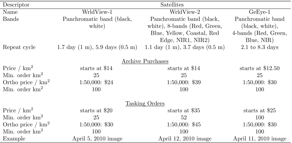
Table 1: Params of some 50 cm resolution satellite sensors used in this study.
Descriptor Satellites
Name WrldView-1 WrldView-2 GeEye-1
Bands Panchromatic band (black, white)
Panchromatic band (black, white), 8-bands (Red, Green,
Blue, Yellow, Coastal, Red Edge, NIR1, NIR2)
Panchromatic band (black, white), 4-bands (Red, Green,
Blue, NIR) Repeat cycle 1.7 day (1 m), 5.9 days (0.5 m) 1.1 day (1 m), 3.7 days (0.5 m) 2.1 to 8.3 days
Archive Purchases
Price / km2 starts at $14 starts at $14 starts at $12.50
Min. order km2 25 25 25
Ortho price / km2 1:50,000: $24 1:50,000: $39 1:50,000: $30
Min. order km2 100 100 100
Tasking Orders
Price / km2 starts at $20 starts at $35 starts at $25
Min. order km2 25 52 100
Ortho price / km2 1:50,000: $30 1:50,000: $45 1:50,000: $30
Min. order km2 100 100 100
Example April 5, 2010 image April 12, 2010 image April 11, 2010 image
evolving as researchers develop new knowledge and dis-seminate developments (Pringle et al., 2012). One of the benefits of seeing the area of interest from the space is also the “large picture” aspect of the satellite imagery that allow us to analyze such characteristics of an inci-dent, which cannot be easily observed from the ground, as the spatial arrangements of the size distributions of different elements and their relations to each other. In the case of this study, the imagery of the pattern of de-struction within the crash site of the Polish Air Force One TU-154M plane destruction on April 10, 2010, con-stitutes an example for an analysis of the patterns of de-bris, their displacements, and their spatial distribution in relation to the available literature on the subject, as well as any related to the incident background in the environmental changes, or human activities, in the area of interest.
Finally, the satellite imagery has its role in the anal-ysis of the appearance and the objects that could be observed from space. It does not allow for any detailed analysis of materials nor does it give unequivocal de-scription of the observed materials. For this reason the satellite imagery analysis is seldom the only means that are used for investigating such incidents as destruction or disturbances, which call for on ground measurements and inspections. Just as a detection of forest fire, hurri-cane, or insect infestation, a detection of any unplanned and potentially undesirable human activities has to be investigated on ground with help of specialized groups of professionals trained in dealing with any given situation.
Thus, for example, an unidentified dumping in the for-est may call for an invfor-estigation with help of chemists, toxicologists or radiologists, to investigate the possibil-ity of toxic waste presence, which would make it illegal as opposed to forest litter raking, which may be a result of permissible activities of local residents.
Objectives
The primary objective of this study was to demon-strate an investigation using satellite images for micro-detail land monitoring and disturbance detection with respect to a site with an important but potentially uncanny development around an incident of interest, whereby the incident of interest was the Polish Air Force One TU-154M plane destruction on April 10, 2010. The secondary objective of this study was to demonstrate usefulness of other seemingly unrelated to land manage-ment scientific inquiries stemming from the image analy-sis observations, for finding answers relating to the above said investigation without sufficient direct evidence or accounts for forming reliable answers.
2
Materials and Data
Table 2: From Apollo Mapping satellite image reseller: available images 0.5 m and 0.6 m (QuickBird only) res-olution taken over the Smolensk airport between 2007 and 2010.
Image type Cloud % Date WorldView-1 0 29-Jun-10 WorldView-1 0 25-Jun-10
GeoEye-1 0 25-Jun-10
WorldView-1 9 21-Jun-10
GeoEye-1 73 9-May-10
WorldView-1 5 14-Apr-10 WorldView-2 0 12-Apr-10
QuickBird 0 12-Apr-10
GeoEye-1 0 11-Apr-10
GeoEye-1 0 9-Apr-10
WorldView-1 11 5-Apr-10 WorldView-1 0 26-Jan-10 QuickBird 100 27-Oct-09 QuickBird 100 12-Oct-09
GeoEye-1 79 25-Jul-09
GeoEye-1 87 25-Jul-09
GeoEye-1 91 6-Jul-09
GeoEye-1 93 6-Jul-09
WorldView-1 98 24-Jun-09
GeoEye-1 71 14-Jun-09
QuickBird 0 31-May-09
QuickBird 0 25-Apr-09
WorldView-1 78 27-Dec-08 WorldView-1 100 14-Dec-08
QuickBird 14 1-Nov-08
WorldView-1 22 5-Apr-08 WorldView-1 100 22-Feb-08 WorldView-1 100 9-Feb-08
QuickBird 0 30-Oct-07
QuickBird 97 25-Oct-07
QuickBird 100 19-Sep-07
for this location for other dates prior to April 2010. Ta-ble 1 lists the params of the relevant satellite sensors from which we purchased the imagery whereas Table 2 lists results of data query searching for available high-resolution images in the timeframe of 2007 to 2010. Fig-ure 1 shows the areas close to the airport for which we were able to find satellite images for the timeframe of our interest. Figure 3 shows the exact placement of each considered scene in relation to our area of interest. Not all the available imagery of interest was covering the de-sirable polygons. The image taken on April 9, 2010 was covering only the West side of the airport, and eventu-ally it proved irrelevant in course of the analysis.
Other available images included GeoEye IKONOS im-ages of 1m resolution that were taken on: 13-Jun-07, 13-Jun-07, 29-Oct-01; SPOT5 satellite images of 2.5 m
Figure 1: The polygons covered by the purchased im-agery.
and 5 m resolutions taken on: 23-May-10, Jul-09, 4-Jul-09, Oct-08, Oct-08, Oct-08, Oct-08, 22-Oct-08, 22-22-Oct-08, 26-Jul-08, 26-Jul-08, Jun-08, 19-Jun-08, 19-19-Jun-08, 19-19-Jun-08, 19-19-Jun-08, 19-19-Jun-08, 08, 3-08, 3-08, 3-08, 3-08, 3-Jun-08, 28-Jul-07, 28-Jul-07, 28-Jul-07, 28-Jul-07, 28-Jul-07, 28-Jul-07, 12-Jun-07, 12-Jun-07, 12-Jun-07, 12-Jun-07, 12-Jun-07, 12-Jun-07, 25-Sep-06, 25-Sep-06, 25-Sep-06, 25-Sep-06, 14-Sep-06, 14-Sep-06, 14-Sep-06, 14-Sep-06, 14-Sep-06, 14-Sep-06, 24-Apr-04, 24-Apr-04, 25-Oct-03, 25-Oct-03; and SPOT4 satellite images of 10 and 20 m resolutions taken on: 30-Apr-10, 4-Apr-10, 9-Mar-10, 11-Feb-9-Mar-10, 29-Apr-09, 29-Apr-09, 24-Nov-08, 25-Oct-08, 25-Oct-25-Oct-08, 7-Sep-25-Oct-08, 7-Sep-25-Oct-08, 26-Jun-25-Oct-08, 26-Jun-25-Oct-08, 5-May-08, 5-May-08, 21-Jan-08, 21-Jan-08, 29-Jan-07, 29-Jan-07, 23-Jan-06, 29-Oct-05, 29-Oct-05, 29-Oct-05, 14-Aug-98, 14-Aug-98, 22-Apr-98, 22-Apr-98, neither of which were considered in our research.
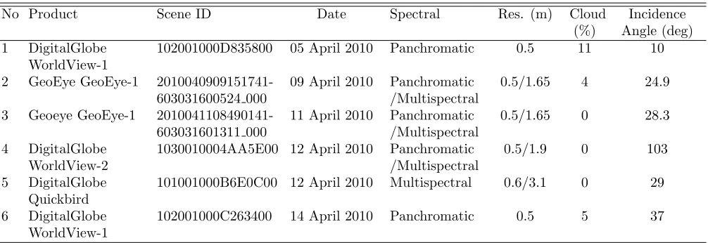
For the purpose of this study, we submitted our data queries through Apollo Mapping’s Image Hunter web application. The data search centered on the crash site filtered for dates ranging from April 6, 2010 to April 15, 2010 and the maximum resolution, cloud cover, snow cover, and incidence angle yielded in 6 results (Tab. 3). Subsequently, we ordered the panchromatic (0.5 m reso-lution), and the multispectral (1.65 to 3.1 m resolution) data products (where available) with intention of ap-plying resolution merging with image sharpening tech-nology. The raw image delivery method from Apollo Mapping was via FTP in GeoTIFF format.
commer-Table 3: Image Hunter April 5, 2010 through April 15, 2010 query results.
No Product Scene ID Date Spectral Res. (m) Cloud
(%)
Incidence Angle (deg) 1 DigitalGlobe
WorldView-1
102001000D835800 05 April 2010 Panchromatic 0.5 11 10
2 GeoEye GeoEye-1 2010040909151741-603031600524 000
09 April 2010 Panchromatic /Multispectral
0.5/1.65 4 24.9
3 Geoeye GeoEye-1 2010041108490141-603031601311 000
11 April 2010 Panchromatic /Multispectral
0.5/1.65 0 28.3
4 DigitalGlobe WorldView-2
1030010004AA5E00 12 April 2010 Panchromatic /Multispectral
0.5/1.9 0 103
5 DigitalGlobe Quickbird
101001000B6E0C00 12 April 2010 Multispectral 0.6/3.1 0 29
6 DigitalGlobe WorldView-1
102001000C263400 14 April 2010 Panchromatic 0.5 5 37
cial images come from the GeoEye-1 and WorldView-1 and -2 sensors, all 50 cm resolution, as follows:
WorldView-1 image taken on April 5, 2010;
GeoEye-1 image taken on April 9, 2010 (western half of the airport only not including the crash site);
GeoEye-1 image taken on April 11, 2010 (available on Google Earth as April 10, 2010, image);
WorldView-2 image taken on April 12, 2010; (but no QuickBird image also taken about 10 min apart;)
WorldView-1 image taken on April 14, 2010.
While all the above images had resolution of 50 cm the readability of different images varied with the angle they were taken from. Two extreme cases are the image of April 5 and April 14 (Fig. 2). There is also a QuickBird image available for April 12, 2010, but it is inferior to the WorldView-2 image for the same date and we did not purchased it for the analysis; although, we partially describe it in this report.
2.2 Other Data
2.3 Literature on Thin Walled Structures Crushing: There is abundant literature on the subject of thin-walled structures crashing, impacts, and mecha-nisms and patterns of their destruction (e.g., (Abramow-icz, 2003, 2004; Hansen et al., 2000; White et al., 1999) illustrating the patterns and types of destruction of thin-walled structures. Other examples of the literature on this subject include: Wierzbicki and Abramowicz (1983), Wierzbicki and Bhat (1986), and Abramowicz et al. (1997). The literature on thin-walled structures destruction describes consistently patterns of bending,
collapsing, crashing, denting, and ripping. Because of those consistent properties of the thin wall structure structions their type of design is frequently built into de-sign of safety architecture within any potentially crash-ing structures. We used the broad literature review in this area to compare the observed pattern of destruction recorded on the satellite imagery with the expectations of the pattern should look like based on the principles published in the engineering literature.
2.4 Ground photographs: There have been many photographs taken on the scene of the incident, and many of them are available on the on the Internet. Among other the acquired photographic material in-cluded many pictures of the heavy equipment used on the site of the plane crash (see Appendix B).
2.5 Weather data: To have a better understand-ing of the conditions at the time of the incident when considering the large patches of snow and possibility of weather influence on the adverse local conditions, we have downloaded temperature and wind data from http://www.wunderground.com (see Appendix B) for the Smolensk area at 791 m elevation, for the last two weeks preceding the incident between March 27 and April 10, 2010.
3
Methods
finally image comparative analysis. At different stages of image processing we were conducting the visual image analysis comparing the different parts of the crash scene on different images taken at different times, and compar-ing the observed patterns and characteristics against rel-evant descriptions of similar phenomena in the literature (e.g., pattern of destruction and spatial size distribution of the debris).
3.1 Image orthorectification The most important image processing before using the image for any analy-sis is orthorectification, which is adjusting the images to compensate for any distortions due to topographic re-lief, lens distortion, distance differences, and the sensor tilt or the incidence angle. The orthorectification con-sists of geometrical corrections assuring that the scale of the image is both uniform and spatially aligned just as a map. Orthorectified images, unlike the raw images, represent true distances, angles and areas, and can be
Figure 2: From top left: raw image entire scenes taken on April 5, 9, 11, 12 by WorldView-2 and QuickBird, and 14, 2010. The images of April 5, 12 QuickBird, and 14, are showing the worst distortions due to the extreme angles of the sensors to the ground.
overlaid with each other for analysis of time dependent changes in any image represented locations.
The raw satellite images that we purchased from Apol-loMapping had to be orthorectified prior to the analysis. Figure 2 shows the raw images for April 5, 9, 11, 12 and 14, which we processed (Fig. 3) before the comparative analysis between different images could be conducted.
We examined the images for patterns and identified various parts of the scenes that needed individual atten-tion or could be helpful when analyzing separately. Ex-amples included parts of crash site with snow patches and other debris sites that had some similarities in the appearance on the images or in texture and spa-tial distribution of scattered objects (e.g., Fig. 20, Ap-pendix B).
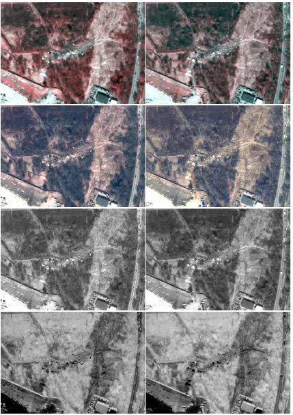
3.2 Multiband resolution merging with image sharpening As mentioned earlier we focused on 0.5 m resolution image analyses, which we wanted to do for all available multi-spectral data. However, only the panchromatic data was available at the 0.5 m resolution (e.g., Fig. 4). The multi-spectral data was available only at lower resolutions of about 2 m. In order to obtain im-ages with 0.5 m resolution for all available multi-spectral bands all the bands with different resolution data had to be merged together with image sharpening technol-ogy to convert the lower resolution bands to the higher resolution.
Figure 4: Half-m panchromatic band.
According with the above we merged the lower res-olution data, which was approximately 2 m multispec-tral data resolution (Figs. 5 A and B) with the higher
resolution 0.5 m panchromatic data (Fig. 4) using the Modified IHS (intensity, hue, saturation) Merge tool (see more examples online at: see more examples online) in the ERDAS1 Imagine 2011 software. The process had to be executed twice on the imagery from April 9, 11, and 12 since this method only processes three (higher resolution) multispectral layers in one pass. Band com-binations 4, 3, 2 (Fig. 5 A) and 3, 2, 1 (Fig 5 B) were pro-cessed in separate runs, yielding two intermediate three-layer data sets. All three three-layers from the 4-3-2 merge and layer 1 from the 3-2-1 merge werelayer stacked to form the final four-band, resolution-merged image data set. The resulting composite images (e.g., Fig 5 C and D) had
Figure 5: Consecutive stages in image sharpening reso-lution merge: a) ‘false-color infrared’ two-m band 4, 3, 2 composite (top-left); b) ‘natural color’ two-m band 3, 2, 1 composite (top-right); c) false-color with the panchromatic half-m resolution-merged output (bands 4, 3, 2) (bottom-left); and d) natural-color with the half-m panchrohalf-matic resolution-half-merged output (bands 3, 2, 1) (bottom right).
the multispectral properties from the higher-resolution data, which originally were 2 m resolutions, while they had the spatial resolution properties of the panchromatic data (Fig. 4) of 0.5 m resolution that we set out to use in our analysis.
3.3 Image processing and param computation We have explored various ways of image processing and
1ERDAS is a trade name of ERDAS, Inc. ERDAS and ERDAS
image manipulation effects. Depending on the types of image processing one can accentuate different elements of the image (Fig. 6). For example, by merging the 2-m multispectral information with the 0.5 m panchromatic resolution of GeoEye we obtain false color infrared im-age showing the green elements appearing red (Fig. 6, row 1). The resolution merged image (2 m multispectral information merged with the 0.5 m panchromatic reso-lution) can be shown as a natural color image. Figure 6, row 2, shows green things green, and color cars with win-dows in the parking lot and the vans with winwin-dows to the south. The panchromatic image (Fig. 6, row 3) shows less detail in color but it appears less busy allowing bet-ter focus on such inventory objects as the plane debris. Even more dramatic polarization of the objects can be achieved with inverted panchromatic images (Fig. 6, row 4).
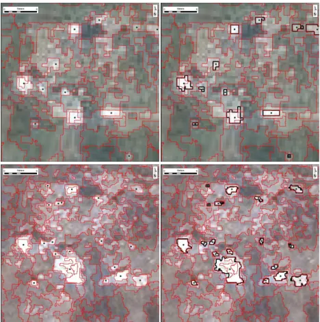
3.4 Image segmentation, delineation, and clas-sification Numerous image enhancement techniques can be applied to each image that may improve or degrade the analysis. These include contrast stretches, image-to-image normalizations, convolution and smoothing, to name just a few. To determine the best segmentation approach we manually delineate well-defined objects then match those results with the auto-mated segmentation results and use them for training the auto-segmentation algorithms. For verification we compare the number and size of the objects for each date.
We explored various options for image segmentation and classification. One example of automatic debris de-lineation is using ERDAS2Imagine region growing tools where the user selects a point and the software expands the polygon automatically. A well-defined object can easily and quickly be determined as something other than natural background. There are image enhancement techniques and image processing methods that, if ap-plied, would improve or degrade the results. None were applied. We used the manual identification of the largest objects on the images from April 11 and 12 to train an automatic classification (Fig. 7), and then applied the trained auto-classification to select the most prominent debris on the crash scenes of the April 11 and 12 images.
3.5 Image auto-comparisons To compare the im-age changes over time we used Thresholding and Blob Analysis. Thresholding enables selecting ranges of pixel values that separate the objects of interest from the background by converting image into a binary image, with pixel values of 0 or 1. All pixels whose value falls within a certain range, called the threshold interval, are
2ERDAS is a trade name of ERDAS, Inc. ERDAS and ERDAS
IMAGINE are registered trademarks of ERDAS, Inc.
Figure 7: Training of the auto segmentation on images from April 11 (top) and 12 (bottom) with the predefined (left) and trained (right) estimates.
set to 1, and all other pixel values in the image are set to 0.
A blob (binary large object) denotes an area of adja-cent homogenous or similar pixels. The pixels in blobs have value of 1, while the rest of the pixels have values of 0. Blob analysis are processing operations and func-tions analyzing information about any shape objects in the image based on various params, such as shape and size of the objects. The information produced by blob analysis can be the size of blobs, their quantity, spatial characteristics, and placement, and cluster and distri-bution characteristics. Such analysis are used in many machine vision functions from detecting welding defects on construction frames to detecting soldering defects on electronic boards.
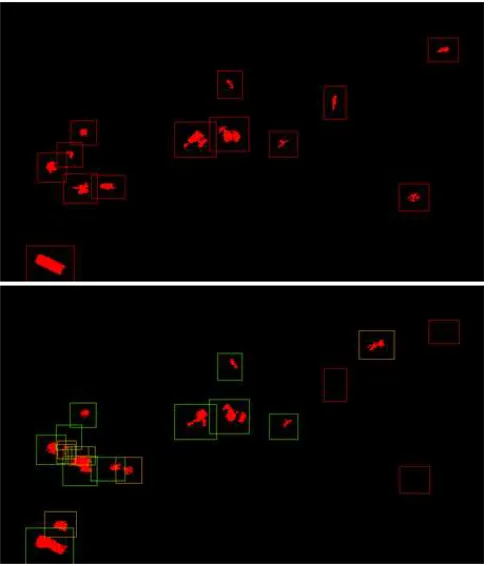
Figure 8: Example of automated image correlation pro-cessing: both images are segmented and then the tar-get image (bottom) is compared with the source im-ages (top) and missing object locations are marked with red squares while new objects are marked with yellow square.
of interest in the process of the image correlation anal-ysis. Subsequently, the bounding box pattern is com-pared between different images and placed in the target images. Since each image has its own blobs and boxes, the source box pattern of blobs is put into a search loop looking for a blob of a similar size in the target image. If the search finds the blob then it displays the blob’s bounding box in green. If a blob is present in the source image, then the algorithm searches for similar blob in the target image in a specific region around its origi-nal location. The result of the search is one of the two conditions:
1. New blobs appear in the target image; or
2. Existing blobs disappear from the target image.
At this point an analyst needs to verify if there is a dis-placement of larger objects or if some smaller objects, which are not visible in the source image could be piled up and forming a larger object with an identifiable ap-pearance in the target image. To distinguish between the different type of situations, we marked on the tar-get image three types of bounding boxes. Green boxes
denote the objects present in the source images at sim-ilar locations as in the target images. The yellow boxes denote new blobs, which were not present in the source images. The locations of the missing objects are marked with the red bounding boxes. To find the correspon-dence between a missing blob and nearest images, the algorithm finds the nearest blobs which of similar sizes and dimensions and analyzes them. To find the exact match, the algorithm looks for the best match among the candidate blobs considering the size dimensions and distance from the original position on the source and target images.
4
Results
4.1 Satellite presence and imagery availability TM images were not very useful in the analysis mainly providing an idea about the regional high frequency of clouds. In conjunction with the weather data, the TM images may be useful in determining that the high level of cloudiness in the considered region was not misrepre-sented by the selection of the available images. No analy-sis of vegetation or soil moisture could be conducted with the level of cloudiness present in the TM images avail-able for the time window of interest. We have looked for images from various sensors for the time and location of interest. Cloud-free (less than 20 of clouds) images available from the incident site include about one image per year on average between the years 2003 and 2010. In the same timeframe, there are 22 images for this lo-cation with high cloud coverage (Tab. 2). Overall, it seems that from a historical perspective year 2010 was statistically an exceptionally cloud-free year in this area (compare cloud covers in Tab. 2). Not a single cloudy image is available for the time between October 2009 and May 2010, and only one image out of total of 12 im-ages in 2010 was captured during high cloud cover. By comparison, in 2009 eight out of 10 images and in 2008 six out of seven, images captured high clouds covers. Consequently, there is relatively few cloud free images available around the Smolensk area of any of the high-resolution sensors since the year 2002. Nevertheless, immediately prior to the time of incident of April 10, 2010, and immediately after the incident, there was an increased presence of the high-resolution sensors satel-lite activities. The high-resolution satelsatel-lite images taken in this region near the incident time covered the dates of April 5, 9, 11, two satellites on 12, 14, all practically cloud-free, and more after that; although, the image of April 9 covers only the west site of the airport and it does not reach the crash area.
agery, with help of different image transformation meth-ods, such as inverting the images, revealed much more useful observations (Fig. 9). The main observations on the consecutive crash scenes start with noticing that the scene of April 5 had almost no big areas of high re-flectance, such as snow patches, that were subsequently replaced by dark (wet) areas. Figure 9 has the major areas of high reflectance marked with red ellipsoids that are marked on all subsequent images as well. It seems to be a quite an extraordinary coincidence that the major-ity of the large high reflectance areas were subsequently replaced on the image of April 11 by accumulations of major plane crash debris residing on seemingly dry (light) ground (Fig. 9 and 10, top left and center). The seemingly dry ground (light reflectance in places of the snow areas replaced by the crash) could be explained if the areas of crash were in these locations sprayed with foam, which seem to be occasionally done on the crash site (e.g., Appendix B, Fig. 19). However, most of the spraying activities recorded on the site were with wa-ter houses that would make the ground even more wet (darker). Most of the other high reflectance patches on April 5 scene were either in areas such as driveways, where the snow gets shoveled sideways, or they were partly concealed from wind by woody shelters where they were subsequently replaced on the image of April 11 by wet (dark) areas from melting snow.
The visual analysis was the most effective though, when we conducted detailed inspections on of various elements on the images in isolation from the rest of the image. For example, Figure 10 shows three example areas that we have compared on the 4 consecutive pic-tures from April 5, 11, 12, and 14. The figure shows quite readily the irregularities that big patches of high reflectance in the crash area convert over time into what seems to be ground patches, even though there is wet ground where there was no snow in the crash area, and there is always wet ground there was snow outside of the crash area.
4.3 Thin-walled structures destruction patterns When the images were zoomed in and inverted for easier interpretation of the plane debris (Fig. 11) the images show a strong pattern of the debris with the smallest parts in the middle and the largest parts thrown out on the perim of the crash area, which is inconsistent with the descriptions of the destruction patterns of thin wall structures (Abramowicz, 2003, 2004; Hansen et al., 2000; White et al., 1999), and which indicates that there were side forces throwing the parts away from the impact point.
4.4 Segmentation and image correlation analy-sis Following the visual analysis, we proceeded to the
Figure 11: Polarized images show more vividly the pat-tern of destruction that is inconsistent with the engineer-ing literature on the subject, because the large objects are thrown out to the perim and the center contains the smallest debris.
Table 4: Statistics for the sample manual, unsupervised and trained selections of polygons in different types of segmentations applied to the April 11 and 12, 2010 images.
Type of selection Manual Selection Auto-selection Trained Auto-selection Statistic April 11 April 12 April 11 April 12 April 11 April 12
Number of polygons 28 44 620 1251 25 42
Mean polygon area (m2) 6.82 5.89 40.22 19.93 14.11 6.32
Minimum polygon area (m2) 0.44 0.39 0.47 0.48 2.48 0.85
Maximum polygon area (m2) 46.07 43.36 393.44 19.38 50.99 34.94 Standard deviation of area (m2) 9.99 9.39 60.15 25.11 14.26 6.96
Figure 12: Trained auto-selection of polygons on the crash area sends up selecting most of the bigger parts scattered mainly around the perim of the site.
the Stokes’ Law the heaviest pieces to the farthest, drove the destruction.
The image correlation analysis reviled active displace-ment of various plane eledisplace-ments (Fig. 13). The changes and moving the major parts from their original locations to new locations started from day one after the crash. Some elements were moved to new locations, left there, and subsequently reported as situated in the new loca-tions as the matter of the original crash results.
We base the above inference on the following logic. Let define the distance for a traveling object asWe base the above inference on the following logic. Let define the distance for a traveling object asx, a function of an initial distancex0, initial velocityv0, accelerationa, and the timet. Symbolically:
x=x0+v0t+
at2
2 (1)
Then, we assume that: x0 = 0; based on the 2nd New-ton’s Lawa=−F/m, whereFis the force acting on the object, andmis the mass of the object, which is a func-tion (m = gαr3) of density (g), the solid object shape dependent constant (α), and the solid object radius (r). These substitutions results in:
x=v0t−
F gαr3
t2
2. (2)
Figure 13: Differential images showing from top: ele-ments that appeared on April 12 as compared to April 11 image; elements that disappeared on April 12 as com-pared to April 11 image; elements that disappeared on April 14 as compared to April 11 image.
its surface. This regularity is obvious to anyone who ever attempted to throw together sand with rocks, or flower with grain; and it is so dependable that it is com-monly implemented in construction and manufacturing standards and testing measurement protocols (e.g., BS EN 196-6:2010 Methods of testing cement).
In physics the Stokes’ Law defines the drag force (F) acting on the solid objects traveling in fluid environment as the function of the fluid viscosity (η), velocity (v), and the solid object radius (r):
F = 6πηvr, (3)
which substituted forF in equation (2) for the traveled distance, results in:
x=v0t− 6πηvr
gαr3
t2
2 =v0t−βvt 21
r2, (4)
whereβis a constant. To define the relationship between the solid object size and its travelled distance we take the derivative of eq. (4) with respect tor, which results in:
dx
dr =−βvt
2·(−2)r−3= 2βvt 2
r3 >0, (5) which concludes this demonstration illustrating that larger objects (with larger values of r) would travel larger distances dx/dr if pushed with the same initial velocity, which would be the case during an explosion occurring insight a thin-walled structure where the ex-panding the gazes would create a uniform pressure on all insight surfaces of the structure disintegrating into pieces of various sizes.
4.5 Reporting of the altered debris positions in government reports, media and Internet Record-ing the main changes in the positions of the largest el-ements on images from April 11 and 12, we notice that the crash scene was not only manipulated on the site, which could have been a matter of urgency in moving various elements, but that the manipulated early posi-tions of the elements have been subsequently reported by the government agencies as the allegedly accurate posi-tions of the plane crash debris. Figure 14 (top image) shows the figure of the crash scene that was published in the MAC report with a sample correction in white ellip-soids circling the misplaced elements and arrows point-ing their original locations based on the April 11 satellite image. Figure 14 (middle and bottom images) shows the published in the Miller report pictures of the crash scene with our corrections in the forms of yellow ellipsoids and arrows as per description above.
Figure 14: MAC report p. 87, Fig. 35 (top), and Miller report p. 18, Fig. 1 (middle and bottom), showing the April 12 image as the original crash scene – the white and yellow arrows point to the original locations of the parts.
5
Discussion
Using satellite imagery is a very powerful way of gath-ering information on land monitoring and disturbance detection. Depending on the availability of various types of images and their resolution, an analyst can not only be very effective in the current state of the word analy-sis, but also can investigate past events that might have not been noticed, recorded, or investigated in a prompt or appropriate manner at the time when they took place.
The lack of large snow areas on the image of April 5, 2010 is not a surprise because since March 27, 2010 the weather in Smolensk was relatively warm and the tem-peratures were above freezing, so much snow would have melted. The presence of the large snow patches where the crash site was located could be seen as peculiar given
the minimal amount of snow throughout the rest of the scene. The coincident of major plane parts crashing on these rare and somewhat peculiar snow patches is in-triguing, and the fact that these major snow patches left dry ground under them is rather strange unless these patches where placed on some kind of sand pits, there was a long and persistent fire at these locations, or pos-sibly ground crews visited these places and shoveled and trucked away the snow before it melted. There is no cer-tainty that the high reflectance areas were actually cre-ated by snow, since any high reflectance objects, such as for example white or silver tarps, would be represented on satellite images in a similar way, but that would not change the peculiarity of the situation that the plane crashed on those very areas.
The analysis of the satellite images showed that the crash scene was manipulated and all the plane debris were moved around and removed from the site in a speedy manner. The results of the crash site changes were captured by the satellite image taken on April 12 and published by both Polish and Russian government official versions of the alleged facts of the incident. The official Russian government MAK (http://www.mak.ru/english/info/tu-154m 101.html) report (Interstate Aviation Committee, 2011a,b) contained misinformation including a number of in-accuracies along with the plane crash altered site illustration erroneously claimed to be correct. Following publication of the Russian official report, the Polish government issued the Miller report (CINAA, 2011), which contained the same April 12 image, proliferated through five graphs on three pages. Moreover, the same error was subsequently proliferated not only in published Russian books subsequently translated and published in Polish language, but also even by other Polish media and knowledge institutions, such as the Polish independent newspaper “Gazeta Polska” and the website http://wikipedia.pl. Both of the later two outlets publicize the satellite image from April 12 as the official account of the original crash scene (i.e., http://bi.gazeta.pl/im/3/7765/m7765863.jpg).
The Wikipedia entry at the URL
http://en.wikipedia.org/wiki/2010 Polish Air Force Tu-154 crash gives the link “Satellite photo of the crash site”, which links to the satellite image of April 12 residing on the website of a Polish newspaper “Gazeta Polska”. An irony of this predicament is that “Gazeta Polska” is a newspaper dedicated to refuting and renouncing many of the accounts provided by the official government sources.
6
conclusions
• even though Google Earth does not contain images for the Smolensk area from between 2007 and 2010 there were quite a few images taken during that timeframe over this area, but they show high fre-quency (up to 80%) of clouds in years 2007–2009, and relatively low frequency (about 10%) of clouds in year 2010;
• the frequency of the high resolution satellite im-agery captured around this airport on the dates of April 5, 9, 11, 12, and 14, 2010, is intriguing given that the satellite tasking ordinarily takes two to four weeks lead time to order imaging over a spe-cific area;
• following warm weather there were few large patches of high reflectivity in the larger area around the Smolensk airport, typically created by accumu-lations of snow, and the larger of the few patches became the exact locations of major plane crash de-bris;
• a few large patches of snow-like high reflectivity ground in the middle of the crash scene did not leave wet ground, signified by dark spots from the snow melting despite generally poorly drained swampy surroundings and no reported major fires;
• the pattern of the plane debris found on the ground following the catastrophe when compared with the engineering literature on thin-walled struc-tures crash destruction patterns was not consistent with expectations associated with a plane crash, but rather was suggestive of an above-ground plane ex-plosion;
• the scene and the plane debris were manipulated over time during the very initial period after the destruction, and the changes to the crash scene dur-ing the few days after the incident were out of the ordinary;
• the altered (manipulated) crash scene became the basis for erroneous information proliferating in pub-lished by the Russian and Polish governments re-ports and by media and Internet-based knowledge bases such as the Wikipedia;
• given the extraordinary amount of heavy equipment activities (as inferred from the point above) on the site it is unclear why the numerous heavy equipment vehicles present were not recorded on any of the satellite images from April 11, 12, or 14, 2010;
• finally, given the findings of this study, it is rec-ommended that the crash scene and all the de-bris be carefully examined by material scientists,
chemists, forensic geoscience scientists, and other experts looking for explanations of the irregulari-ties concluded in the course of this study.
Acknowledgements
This study was sponsored by the D.B. Warnell School of Forestry and Natural Resources, University of Geor-gia, Athens, GA, USA. Many thanks are due to prof. Piotr Witakowski, who invited this study and who was very helpful in all the dealings with the Smolensk Confer-ence organization and with administrating the relevant research reviews. We would like to thank also the five anonymous reviewers and the manuscript editors who provided helpful comments on the earlier version of this manuscript.
References
Abramowicz, W. 2003. Thin-walled structures as impact energy absorbers. Thin-Walled Structures. 41: 91– 107.
Abramowicz, W. 2004. An alternative formulation of the FE methodfor arbitrary discrete/continuous models. International Journal of Impact Engineering. 30(8-9): 1081–1098.
Abramowicz, W, Jones, N. 1997. Transition from initial global bending to progressive buckling of tubes loaded statically and dynamically. International Journal of Impact Engineering. 19(5-6): 415–437.
Alcaraz-Segura, D, Cabello, J, Paruelo, JM, Delibes, M. 2008. Trends in the surface vegetation dynamics of the national parks of Spain as observed by satellite sensors. Applied Vegetation Science. 11(4): 431–440.
Asner, GP. 2009. Tropical forest carbon assessment: In-tegrating satellite and airborne mapping approaches. Environmental Research Letters. 4(3): 034009.
Celik, T, Tjahjadi, T. 2010. Image resolution enhance-ment using dual-tree complex wavelet transform. IEEE Geoscience and Remote Sensing Letters. 7(3): 554–557.
Chen, HY, Leou, JJ. 2012. Multispectral and multireso-lution image fusion using particle swarm optimization. Multimedia Tools and Applications. 60(3): 495–518.
Choi, J, Yeom, J, Chang, A, Byun, Y, Kim, Y. 2013. Hybrid pansharpening algorithm for high spatial res-olution satellite imagery to improve spatial quality. IEEE Geoscience and Remote Sensing Letters. 10(3): 490–494.
Cieszewski, CJ, Liu, SB, Lowe, RC, Zasada, M. 2011. Spatially explicit biomass sustainability analysis for bioenergy mill siting in Georgia, USA. The Open For-est Science Journal. 4(1): 2–41.
Cieszewski, CJ, Zasada, M, Borders, BE, Lowe, RC, Zawadzki, J, Clutter, ML, Daniels, RF. 2004. Spa-tially explicit sustainability analysis of long-term fiber supply in Georgia, USA. Forest Ecology and Manage-ment. 187(2-3): 349–359.
CINAA (Committee for Investigation of National Avi-ation Accidents) KBWL. 2011. Final Report on the examination of the aviation accident no 192/2010/11 involving the Tu-154M airplane, tail number 101, which occurred on April 10th, 2010 in the area of the Smolensk North airfield, Warsaw (In En-glish). Available online at: http: //mswia.datacenter-poland.pl/FinalReportTu-154M.pdf. Last accessed on Feb. 12, 2013.
Daliakopoulos, IN, Grillakis, EG, Koutroulis, AG, Tsa-nis, IK. 2009. Tree crown detection on multispectral VHR satellite imagery. Photogrammetric Engineering and Remote Sensing. 75(10): 1201–1211.
Demirel, H, Anbarjafari, G. 2010. Satellite image reso-lution enhancement using complex wavelet transform. IEEE Geoscience and Remote Sensing Letters. 7(1): 123–126.
Demirel, H, Anbarjafari, G. 2011. Discrete wavelet transform-based satellite image resolution enhance-ment. IEEE Transactions on Geoscience and Remote Sensing. 49(6): 1997–2004.
Franke, J, Navratil, P, Keuck, V, Peterson, K, Siegert, F. 2012. Monitoring fire and selective logging activi-ties in tropical peat swamp forests. IEEE Journal of Selected Topics in Applied Earth Observations and Remote Sensing. 5(Special Issue): 1811–1820.
Hanssen, AG, Langseth, M, Hopperstad, OS. 2000. Static and dynamic crushing of square aluminium extrusions with aluminium foam filler. International Journal of Impact Engineering. 24(4): 347–383.
Hu, MG, Wang, JF, Ge, Y. 2009. Super-resolution recon-struction of remote sensing images using multifractal analysis. Sensors. 9(11): 8669–8683.
Interstate Aviation Committee (MAK). 2011a. Final Re-port on results of investigation of aviation accident in-volving the Tu-154B-2, tail number RA-85588, airport Surgut, on January 1, 2011. (In Russian).
Interstate Aviation Committee (MAK). 2011b. Fi-nal Report on the investigation of air accident of Tu154M registration number 101 of the Republic of Poland. Moscow, 2011. Available online at http: //www.mak.ru/russian/investigations/2010/tu-154m 101/finalreport eng.pdf, last accessed on Feb. 11, 2013.
Iqbal, MZ, Ghafoor, A, Siddiqui, AM. 2013. Satellite im-age resolution enhancement using dual-tree complex wavelet transform and nonlocal means. IEEE Geo-science and Remote Sensing Letters. 10(3): 451–455.
Liu, G, Sun, X, Fu, K, Wang, HQ. 2013. Aircraft recog-nition in high-resolution satellite images using coarse-to-fine shape prior. IEEE Geoscience and Remote Sensing Letters. 10(3): 573–577.
Liu, S, Cieszewski, CJ. 2009. Impacts of management intensity and harvesting practices on long-term forest resource sustainability in Georgia. Mathematical and Computational Forestry & Natural-Resource Sciences. 1(2): 52–66.
Liu, S, Cieszewski, CJ, Lowe, R, Zasada, M. 2009. Sensi-tivity analysis on long-term fiber supply simulations in Georgia. Southern Journal of Appled Forestry. 33(2): 81–90.
Lowe, RC, Cieszewski, CJ, Liu, S, Meng, Q, Siry, J, Zasada, M, Zawadzki, J. 2009. Assessment of stream management zones and road beautifying buffers in Georgia based on remote sensing of various ground inventory data. Southern Journal of Applied Forestry. 33(2): 91–100.
Ma, JL, Chan, JCW, Canters, F. 2010. Fully au-tomatic subpixel image registration of multiangle CHRIS/Proba Data. IEEE Transactions on Geo-science and Remote Sensing. 48(7): 2829–2839.
Meng, Q., C.J. Cieszewski. 2006. Spatial clusters and variability analysis of tree mortality. Physical Geog-raphy 27(6): 534–553.
Meng, Q, Cieszewski, CJ, Madden, M. 2009a. Large area forest inventory using Landsat ETM plus: A geosta-tistical approach. ISPRS Journal of Photogrammetry and Remote Sensing. 64: 27–36.
Meng, Q, Cieszewski, CJ, Madden, M. 2007a. A linear mixed-effects model of biomass and volume of trees us-ing Landsat ETM+ Images. Forest Ecology and Man-agement. 244: 93–101.
Meng, Q, Cieszewski, CJ, Madden, M, Borders, BE. 2007b. K Nearest Neighbor method for forest inven-tory using remote sensing data. GIScience and Remote Sensing 44: 149–165.
Moller, M, Wittman, T, Bertozzi, AL, Burger, M. 2012. A variational approach for sharpening high dimen-sional images. Siam Journal on Imaging Sciences. 5(1): 150–178.
Olsson, P-O, Jonsson, AM, Eklundh, L. 2012. A new invasive insect in Sweden - Physokermes inopinatus: Tracing forest damage with satellite based remote sensing. Forest Ecology and Management. 285: 29– 37.
Pelletier, J, Codjia, C, Potvin, C. 2012. Traditional shift-ing agriculture: Trackshift-ing forest carbon stock and bio-diversity through time in western Panama. Global Change Biology. 18(12): 3581–3595.
Pringle, JK, Ruffell, A, Jervis, JR, Donnelly, L, McKin-ley, J, Hansen, J, Morgan, R, Pirrie, D, and Harrison, M. 2012. The use of geoscience methods for terrestrial forensic searches. Earth-Sciences Reviews. 114: 108– 123.
White, MD, Jones, N, Abramowicz, W. 1999. A theo-retical analysis for the quasi-static axial crushing of top-hat and double-hat thin-walled sections. Interna-tional Journal of Mechanical Sciences. 41: 209–233.
Wierzbicki, T, Abramowicz, W. 1983. On the crushing mechanics of thin walled structures. Journal of Ap-plied Mechanics. 50: 727–734.
Wierzbicki, T, Bhat, S. 1986. A note on shear effects in progressive crushing of prismatic tubes. S.A.E. Tech-nical Series, Paper No. 860821.
Zawadzki, J, Cieszewski, CJ, Zasada, MJ. 2004a. The use of geostatistical methods for remote-sensing based determination of inventory measures and biophysical params of forests. Sylwan. 3: 51–62. (In Polish).
Zawadzki, J, Cieszewski, CJ, Zasada, MJ. 2004b. Use of geostatistical methods for classification of forest ecosystems using satellite imagery. Sylwan. 2: 26–41. (In Polish).
Zawadzki, J, Cieszewski, CJ, Zasada, MJ. 2005a. Semi-variogram analysis of Landsat 5 TM textural data for loblolly pine forests. Journal of Forest Science. 51(2): 47–59.
Zawadzki, J, Cieszewski, CJ, Zasada, MJ, Lowe, RC. 2005b. Applying geostatistics for investigations of for-est ecosystems using remote sensing imagery. Silva Fennica. 39: 599–618.
Zhi-Ying, Z, X. De-Zhonga, Z. Xiao-Nong, Z Yun, L Shi-Jun. 2005. Remote sensing and spatial statistical analysis to predict the distribution of Oncomelania hupensis in the marshlands of China. Acta Tropica. 96: 205–212.
Appendix A: Types of imaging sensors
and free satellite images
Many sources of satellite data are available and an excellent overview of different satellite sensors is at http://www.satimagingcorp.com/satellite-sensors.html. The USGA website contains the various current satel-lite products at: http://eros.usgs.gov/. . . Products. Different examples of the satellite imagery are at http://www.satimagingcorp.com/gallery.html. The commercially available satellite images can be also browsed on various satellite image reseller sites, such as DigitalGlobe and ApolloMapping.
Figure 15: LTM5 images from April 8 and 24, 2010 (top and mid-top), ETM7 image taken on April 16, 2010 (bottom-mid); and LTM5 image taken on April 15 (bot-tom).
Figure 16: Free images available on the Internet. Top to bottom: Google Earth image from October 2007 and April 11, 2012 (labeled in Google Earth as April 10); DigitalGlobe image from April 12, 2012; and Google Earth image from Jun. 10, 2010.
Figure 17: Some of the heavy equipment operating on the crash scene on April 11-14, 2010, on the crash site by Dr. Jan Gruszynski.
ALOS – high resolution, global land observation data.
ASTER – monitoring cloud cover and other environ-mental patterns.
CARTOSAT-1 – mainly intended for cartographic ap-plications in India.
CBERS-2 – various mapping of environmental objects.
FORMOSAT-2 – multipurpose satellite for remote sensing and scientific observations.
GeoEye-1 – diverse array of applications.
IKONOS – high-resolution operated by GeoEye.
LANDSAT-7 – multispectral scanning or earth re-sources.
Pleiades-1 – high-resolution orthorectified color data.
Figure 18: Temperature, dew point, baromet-ric pressure, and wind data for Smolensk, Rus-sia, March and April, 2010, downloaded from http://www.wunderground.com/ website.
RapidEye – constellation of five satellites geospatial information for daily image data.
SPOT-5 and SPOT-6 – medium-scale mapping.
WorldView-1 – high-capacity panchromatic imaging system.
WorldView-2 – includes pan-sharpened, multispectral imaging.
WorldView-3 – a high-resolution satellite sensor from GeoEye (expected in late 2014).
Satellite imagery can be purchased through different reselers specializing in a variety of selections and prod-ucts. Table 5 contains many of the resellers listed on the USGA website with their names, Internet links, and physical addresses.
The free imagery that we considered in this study included some TM and ETM images and some other higher resolution imagery downloaded from GlobalDig-ital and Google Earth. The TM and ETM imagery is possibly the most widely used due to its broad system-atic coverage, frequent cycles, and free of charge avail-ability. Even though the TM and ETM images have 27.5 m resolution, they are useful for many diverse problems with examples ranging from even such unlikely applica-tions as analysis of snail distribution in China marsh-lands (Zhi-Ying et al., 2005) to compilations of national inventories.
There was no cloud-free Landsat 5 TM or Landsat 7 ETM imagery available for the considered time-frame around the April 10, 2010, date. There are
Figure 19: White powder spraying activity on the plane crash site. Photo from gazeta.pl.
two path/rows for this, Smolensk, Russia, area. Path 181 row 22 has two LTM5 images from April 8 and 24, 2010 (Fig. 15, top and mid-top), and one image ETM7 taken on April 16, 2010 (Fig. 15, bottom-mid). Path 182 row 22 has two LTM5 images taken on April 15 (Fig. 15, bottom) and February 5, 2010, which was not acquired. One DigitalGlobe image captured on April 12, 2010 (Fig. 16, mid-bottom) is available for free and it can be downloaded from http://store.digitalglobe.com/russia—smolensk-crash-p237.aspx. Finally, Google Earth provides access to some processed imagery taken on May 27, 2005, October 29, 2007 (Fig. 16, top), June 24, 2010 (Fig. 16, bottom), and the controversial image marked in Google Earth as taken on April 10, 2010 (Fig. 16, mit-top), which according to its metadata was actually taken on April 11 8:49 am Greenwich Mean Time (GMT), which is similar to the Coordinated Universal Time (UTC), while Google might be displaying for example the Alaska time (i.e., 10.04.2010, 23:49 UTC-10:00).
Appendix B: Auxiliary data considered
in the image analysis of the Smolensk
incident of April 10, 2010
6.1 Ground photographs: Many ground taken pic-tures of heavy equipment working on the crash site are available on the Internet in forms of both still shots and videos. Figure 17 contains several examples of such pic-tures that were available first-hand to the authors of this article from the author of the pictures.
Table 5: Names, URLs and addresses of resellers listed on the USGA WebSite.
Business Name Location
AGRI IMAGIS Maddock, North Dakota United States 58348
AMEC Earth and Environmental Westford, MA 01886
APPLIED ANALYSIS INC Billerica, Massachusetts United States 01821
ARUNA TECHNOLOGY LTD. Phnom Penh, Cambodia
C S I R/SATELLITE APPLICATIONS CENTRE Pretoria, Gauteng South Africa 0001
COMPUTAMAPS Constantia 7848, South Africa
DIGITALGLOBE, INC. Longmont, Colorado United States 80503
E G S TECHNOLOGIES CORP. Bloomingdale, Illinois United States 60108 EARTH DATA ANALYSIS CENTER Albuquerque, New Mexico United States 87131 EARTH SATELLITE CORPORATION Rockville, Maryland United States 20852 EAST VIEW CARTOGRAPHIC INC. Minneapolis, Minnesota 55305
ENGESAT IMAGENS DE SATELLITES Curitiba, Brazil 80530-060
ERICSSON Inc. Richardson, Texas United States 75080
EURIMAGE S.P.A. Rome 00155, Italy 00155
FOREST ONE INC. Evanston, Illinois United States 60201
G T T NET CORP. Tampa, Florida United States 33685
GEOCARTO INTERNATIONAL CENTRE Hong Kong, China, Peoples Republic of
GEOIMAGE Taringa, Queensland Australia 4068
GEOMART Laramie, Wyoming United States 82072
GEO-RESEARCH Lahore-54700, Lahore - Punjab Pakistan
GEOSERVE B.V. Marknesse, Netherlands
GEOSYS, INC. Plymouth, Minnesota United States 55447
GLOBEXPLORER INC. Walnut Creek, California United States 94598
HYDROBIO Santa Fe, New Mexico United States 87501
I-CUBED Fort Collins, Colorado United States 80524
IMAGELINKS, INC. Melbourne, Florida United States 32934
INFOSTRATA S. A. Belo Horizonte, Mg, Brazil 30112-010
INFOTERRA LTD. Farnborough, Hampshire United Kingdom GU14 ONL
INNOTER Moscow, Russian Federation 115088
ISTAR Sophia Antipolis, France
JEODIJITAL BILISIM TEKNOLOJI LTD. Ankara, Turkey 06510
KOGER REMOTE SENSING Forth Worth, Texas United States 76109
LE GROUPE SYSTEME FORET INC. Quebec City, Quebec Canada GIP 2J3
MADECOR GROUP Los Banos, Phillipines 4031
MAPMART Greenwood Village, CO 80111
NIGEL PRESS ASSOCIATES LIMITED Edenbridge, Kent United Kingdom TN8 6SR
NIVELES S. A. DE C. V. 09360 Mexico Df, Mexico
PACIFIC GEOMATICS LTD. Surrey, British Columbia Canada V4P1R4
PERRY REMOTE SENSING LLC Englewood, Colorado United States 80110
PHOTOSAT INFORMATION Ltd. Vancouver, BC Canada VGE 4A2
PRECISION PARTNERS, INC. Fergus Falls, Minnesota United States 56538
PROSIS S.A. Bogota, Columbia
PT EARTHLINE Cilandak, Jakarta 12310, Indonesia Indonesia
PT. ADINUGRAHA SATELINDO Jakarta 10270, Indonesia
RADARSAT INTERNATIONAL INC. Richmond, British Columbia Canada V6V2J3 RESEARCH & DEVELOPMENT CENTER, SCANEX Moscow, Russia
RESTEC Tokyo, Japan 106-0032
RITRE Corporation Rochester, NY 14624
SERVICIOS SIGIS Caracas, 1071, Venezuela 1080
SILVANA IMPORT TRADING INC. Montreal, Quebec Canada H32 1P7
SOVZOND JOINT STOCK COMPANY Moscow 101000, Russia
SPOT IMAGE CORPORATION Reston, Virginia United States 20191
STAR VISION Ltd. Hong Kong, China
T T I PRODUCTION Nimes, France 30900
Table 6: Weather data on Aprlil 10, 2010, from www.wunderground.com at the Moscow Daylight Time (MSD).
Time (MSD)
Temp.˚C Dew Pt.˚C
Humidity Pressure hPa
Visibility km
Wind Dir
Wind km/h
Events Conditions
1:00 AM 6 -0 52 1025 10 SE 7.2 Mostly Cloudy
4:00 AM 3 -0 72 1025 10 SE 7.2
7:00 AM 0 -1 89 1025 4 ESE 7.2 Mist
10:00 AM 1 1 98 1026 0.5 SE 10.8 Fog Heavy Fog
1:00 PM 3 2 94 1025 4 East 14.4 Mist
7:00 PM 12 -0 31 1023 10 East 14.4 Clear
10:00 PM 7 -1 45 1024 10 Calm Calm Clear
Figure 20: An example of a debris area that has a similar appearance in terms of presence of unidentified debris spatially distributed over a limited space that hasn’t much changed since 2007.
Example of image part with scattered debris in Smolensk that have partly similar appearance to the plane crash site but have not changed much since 2007 as compared with the fast and dramatic changes of the