e-ISSN: 2278-7461, p-ISSN: 2319-6491
Volume 8, Issue 2 [February 2019] PP: 33-54
Optimization of Flow Parameters in Gas Pipeline Network
System (Panhandle-A as Base Equation)
Dr. Mathew, Shadrack Uzoma, Prof (Mrs) O. M. O. ETEBU
Department of Mechanical Engineering University of Port Harcourt Port Harcourt, Rivers State, Nigeria Department of Mechanical Engineering University of Port Harcourt Port Harcourt, Rivers State, Nigeria
Corresponding Author: Dr. Mathew
ABSTRACT: Gas pipeline assets and facilities are capital intensive production assets. Optimization of flow parameters in gas pipelines network system applying the models developed by the researcher is the focus of this work. The developed optimization models background is fundamental Panhandle A equation.
The optimization results for single phase flow of gas in the five gas pipelines system used as case study confirmed that about 10% additional throughput over the normal operational levels could be accommodated by existing gas pipelines in Nigerian terrain. There could also be a drastic 20% to 45% reduction in line pressure drop.
It was discovered in this work that optimization of flow parameters led to drastic reduction in pressure drop along the line and increased flow throughput. It has been established that increased line pressure drop would ultimately lead increased pump and compressor power. As such, higher cost of design, construction and operation of gas pipeline should be the order of the day.
The developed optimization models for flow variables could enable gas pipeline assets and facilities to be designed and operated efficiently; so that our gas reserves could be conserved and deployed for strategic development ofthe nation’s vast gas reserves estimated at 185 trillion standard cubic feet.
Keywords : Assets and Facilities; Capital Intensive; Flow Parameters; Line Pressure Drop; Construction and Operation Costs; Strategic Development; Vast Gas Reserves; Criss-Crossing; Inefficiently Operated and Pipeline Network System.
Nomenclature
G
V
L
V
,
liquid and gas local velocities (m/s)M
V
–- mixture mean flow velocity (m/s) µG—absolute gas viscosity (Pas)A, B, C—virialcoefficients (J/kg)
AR—area ratio
a—Van der Waals pressure correction factor (N/m4) b-- Van der Waals volume correction factor (m3) C—empirical constant
Cp—ratio of static pressure to dynamic pressure
d0—outside diameter of pipe (inches)
D—nominal pipe diameter (cm) d—pipe inner diameter (inches) E—longitudinal weld joint factor
K4—entrance loss coefficient
K5—exit loss coefficient
Kp—pump loss coefficient
Kw, Kp1, Kp2—constants
G
V
L
V
,
liquid and gas average velocities (m/s)
2
/
2
,
2
/
n
2
G
V
n
L
V
liquid and gas acceleration gradients perpendicular to theaxis of the pipe (1/s2)
Z
G
V
Z
L
V
/
,
/
liquid and gas velocity gradients along the axis of the pipe (1/s)L—length of pipeline (km)
m—mass of gaseous constituents (kg)
P1—upstream pressure (bar)
P2—downstream pressure (bar)
P3—average flow pressure (bar)
Pb—base pressure (bar)
Q—flow capacity (m3/s) Qg—gas flow rate (m3/day)
ReNS—Reynolds number at no slip condition
R—individual gas constant (J/kgK) RL, RG—liquid and gas holdup
S—allowable yield stress for pipe (psi)
SG—specific gravity of the liquid relative to water SY—maximum yield stress for pipe (psi)
Tb—base temperature (K)
T—bulk flow temperature (K)
Tol—manufacturers tolerance allowance (m)
t—pipe wall thickness (inches) tth—thread or groove depth (inches)
Vg—gas velocity (ft/s)
V—mean flow velocity (m/s)
W—weight of pipe filled with water (lb/ft) Y, F—derating factors
Z—flow compressibility factor
α2—kinetic energy flux coefficient
λ—volume fraction of gas flowing (m3
/s)
μNS—Absolute viscosity at no slip condition (Pas)
νf—kinematics viscosity of the fluid stream (Pas)
ρG—gas density (kg/m3)
ρL—liquid density (Kg/m3)
ρNS—density at no slip condition (kg/m3)
ρTP—density for two-phase flow (Kg/m3)
∆Pa—acceleration pressure drop (bar)
∆Pec—losses due to enlargement and contraction (bar)
∆Pe—elevation pressure drop (bar)
∆Pent—entrance losses (bar)
∆Pexit—exit losses (bar)
∆Pf—frictional pressure drop (bar)
∆Pft—fitting losses (bar)
∆P—overall pressure drop along the line (bar)
∆Pp—pump losses (bar)
∆Pv—valve losses (bar)
I.
INTRODUCTION
Gas pipeline pressure-flow problem are affected by varieties of factors notably frictional pressure drop and other pressure drops components. These problems inevitably result in the reduction of the operating efficiency of gas pipelines by virtue of reduction in the line throughput and increased pressure drop along the line. It has been established that increased pressure drop will ultimately lead to increased pump power as well as higher cost of design, construction and operations of gas pipelines.
Flow optimization could enable these assets to be put to optimal use throughout their design life. Current gas reserves in Nigeria are conservatively put at approximately 185 trillion standard cubic feet [1]. Therefore, it is imperative that gas facilities be designed and operated efficiently so that available resources could be conserved and deployed for strategic development of the nation’s vast gas resources. To this effect, the researcher has developed optimization models employing Weymouth equation, Panhandle A equation and Modified Panhandle B as the fundamental base equation [2, 3, 4].
Study Significance
The developed optimization models is the first of its kind. Matlab is used in coding the programming algorithm. The programming algorithmic coding is the easy to handle type. It produces optimal results of flow variables in few iteration steps. It is strongly believed that the findings in this work could provide the base for further in-depth research in gas pipeline flow optimization. The focus should be more biased on optimization of flow capacity viz-a-viz the overall pressure drop along a gas pipeline.
Thus the following objectives are imperative of this work: (i) Predictability of performance.
(ii) Efficient utilization and deployment of gas pipeline assets and facilities.
(iv) Design efficiency in sizing gas pipelines and associated equipment.
(v) Greater economy in the design and operation of gas pipelines. (vi) Longer service life to gas pipelines.
Relevant Optimization Models
Friction factor for two phase flow is expressed as :
ln
2
0
.
94
ln
3
0
.
0843
ln
4
444
.
0
)
ln
(
478
.
0
281
.
1
S
G L
R
R
1
The absolute gas viscosity for the mixture of the hydrocarbon constituents of the gas is expressed by [5] :
1
.
8
0
.
27
.
2
6
10
062
.
2
5
10
709
.
1
log
3
10
15
.
6
3
10
188
.
8
5
10
02247
.
1
T
G
G
GHC
The absolute viscosity of nitrogen is given as:
3
2
log
3
10
48
.
8
3
10
59
.
9
5
10
02247
.
1
2
N
n
G
GN
The absolute viscosity of carbon dioxide expressed as:
4
2
log
3
10
08
.
9
3
10
24
.
6
5
10
02247
.
1
2
CO
n
G
GCO
Absolute viscosity of hydrogen sulphide is given as:
5
2
log
3
10
49
.
8
3
10
73
.
3
5
10
02247
.
1
2
H
S
n
G
S
GH
Model for pressure drops along pump and compressor :
4 2 2
2 4 2
1
16
6
1
16
d
K
where
Q
K
Q
d
P
i P
P i P
Kp—Pump constant
ηi=85 % to 97.5 % for most pumps and compressors [6].
Apparentmolecular weight of natural gas on the basis of the mole fractions of thedifferent constituents is expressed as:
7
1
N
i
i
M
i
n
a
M
The gaseous mixture specific gravity is given as:
8
.
air
M
a
M
G
In terms of the pseudo reduced properties, the critical pressure of the gaseous mixture is expressed as:
Ni Ci i
c
n
P
P
1
9
The critical temperature of the mixture is given as:
10
1
Ni Ci i
C
n
T
T
12
.
11
C r
C r
T
T
T
P
P
P
Average gas pressure, P is given by [5] :
13
3
2
2 2 2 1
3 2 3 1
P
P
P
P
P
Gas density is given as:
14
...
...
...
...
...
...
...
...
...
...
...
...
...
...
ZRT
P
G
OPTIMIZATION MODEL BASED ON PANHANDLE- A EQUATION The fundamental Panhandle -A equation is expressed as [7] :
.
day
2.618
cm
0.5394
K
/
0.5394
Km
3
m
is
PA
K
of
unit
the
1.90826;
=
PA
K
(15),
Equation
in
is
it
As
15
6182
.
2
4606
.
0
1
5394
.
0
2
2
2
1
5394
.
0
1
788
.
1
D
G
ZL
T
P
P
f
b
P
b
T
PA
K
Q
Conditions of Application
Panhandle-A flow equation is applicable at moderate flow rates for partially developed turbulent flows and for long transmission lines. Usually the pipe wall is smooth. The flow situation is steady state flow, annular with suspended liquid mists in a two phase flow problem. The range of pipe diameter is greater than twelve inches (12”). The flow situation is annular in nature.
Equation (15) could be re expressed as ;
. day 2.618 cm 0.5394 K / 0.5394 Km 3 m
is P A K of unit the 1.90826; =
P A K 3.43, Equation In
2 P -1 P P
16 .
5394 . 0 6182 . 2 4606 . 0 1 5394 . 0 2 1 5394 . 0 1 5394 . 0 1 788 . 1
6182 . 2 4606 . 0 1 5394 . 0 2 1 2 1 5394 . 0 1 788 . 1
P D
G L
T P P Z
f b
P b T PA K
D G
ZL T
P P P P f
b P
b T PA K Q
2.61825394 . 0 2 1 0788 . 0 2 1 2 2 2 1 2 1 0 4606 . 0 788 . 1 0788 .. 0 1 5394 . 0 5394 . 0 1 5394 . 0 5394 . 0 6182 . 2 5394 . 0 2 1 0788 . 0 2 1 2 2 2 1 2 1 0 4606 . 0 788 . 1 0788 .. 0 5394 . 0 5394 . 0 6182 . 2 5394 . 0 2 1 4606 . 0 5394 . 0 788 . 1 0788 . 0 2 1 2 2 2 1 2 1 0 4606 . 0 0788 . 0 2 1 0 2 1 2 2 2 1 4606 . 0 0788 . 0 4606 . 0 5394 . 0 4606 . 0 5394 . 0 4606 . 0 4606 . 0 4606 . 0 5394 . 0 2 1 2 2 2 1 2 1 0 5394 . 0 5394 . 0 5394 . 0 6182 . 2 5394 . 0 2 1 4606 . 0 5394 . 0 788 . 1
5
.
1
,
18
1
1
5
.
1
1
1
1
03247
.
1
3
2
1
1
1
1
2
3
1
17
1
1
1
D
L
T
P
P
P
P
P
P
M
P
P
T
R
M
M
P
T
K
K
Where
P
f
K
Q
P
f
D
L
T
P
P
P
P
P
P
M
P
P
T
R
M
M
P
T
K
P
f
D
L
T
P
P
G
Z
P
T
K
Q
P
P
P
P
M
P
P
T
R
M
M
P
P
T
R
P
P
P
P
M
M
M
Z
M
M
Z
M
Z
M
Z
G
M
Z
M
G
P
P
P
P
M
P
P
T
R
Z
P
f
D
L
T
P
P
G
Z
P
T
K
Q
a b b PA PA PA a b b PA b b PA a a a a a b b PA
The various pressure drop components in terms of the flow capacity are as follows [5] :
(a) Frictional Pressure Drop, ∆Pf
Where:
L—overall length of pipeline (km)
LL—length of pipe line based on required number of pipes (km)
Lev—equivalent length of valves (km)
Lef—equivalent length of fittings (km)
Lel—equivalent length of elbows (km)
(b) Elevation Pressure Drop, ∆Pe
el ef ev L G G G fL
L
L
L
L
Q
D
L
LQ
D
Q
Q
D
L
LQ
D
Q
D
Q
D
LQ
f
D
LQ
V
D
L
f
P
68 . 1 32 . 0 68 . 0 2 5 2 32 . 0 32 . 0 2 322 . 0 2 5 2 32 , 0 32 . 0 32 , 0 5 2 2 5 2 2 29256
.
0
0112
.
0
1
/
9256
.
0
0112
.
0
1
1157
.
0
0014
.
0
8
8
2
H
g
P
e
(c) Entrance Losses (Pressure Drop), ∆Pen
(d) Exit losses (Pressure Drop), ∆Pex
(e) Pressure Drop Due To Enlargement and Contraction, ∆Pec
(f) Valves Pressure Drop, ∆Pv
(g) Fittings Pressure Drop, ∆Pft
The value assigned to L/D ratio either for the valves or fittings is a function of the type of valve or fitting
in question.
(h) Acceleration Pressure Drop, ∆Pa
(i) Pump Pressure Drop, ∆Pp
The equation for pump pressure drop applies to all types of pumps and compressors, all that need be
known is the isentropic efficiency of the particular pump or compressor.
(j) Overall Pressure Drop, ∆P is expressed as:
19
p
P
ft
P
v
P
ec
P
ex
P
en
P
a
P
e
P
f
P
P
Substituting the various pressure drop components in Equation (3.46);
24 2 2 41 2 2 41
1
8
2
1
Q
D
K
V
K
P
en
2 4 2 51 2 518
2
D
Q
K
V
K
P
ex
n n P P ecQ
K
Q
D
AR
V
P
AR
V
V
P
P
AR
V
V
P
P
C
C
AR
V
P
/ 1 / 1 2 4 2 2 2 2 2 2 2 1 2 2 2 1 2 2 28
1
1
2
/
1
1
2
2
/
1
1
2
2
/
,
1
1
2
2 0.68 0.32 1.68
5 2 32 . 0 32 . 0 2 322 . 0 2 5 2 32 , 0 32 . 0 32 , 0 5 2 2 2 29256
.
0
0112
.
0
1
/
9256
.
0
0112
.
0
1
1157
.
0
0014
.
0
8
2
2
Q
D
L
Q
L
D
Q
Q
D
L
Q
L
D
Q
D
Q
D
Q
L
f
V
D
L
V
D
L
f
P
G ef ef G ef ef G ef ef ef ft
2 4 2 28
2
D
Q
V
P
a
2 4 2 4 2 21
16
1
16
,
Q
D
D
K
Q
K
P
p p p
20 . / 1 / 1 68 .. 1 32 . 0 68 . 0 9256 . 0 32 . 0 68 . 0 9256 . 0 32 . 0 68 . 0 9256 . 0 5 2 1 2 4 2 1 16 5 2 0112 . 0 5 2 0112 . 0 4 2 8 2 1 1 4 2 51 8 4 2 1 2 41 8 4 2 8 5 2 0112 . 0 / 1 / 1 68 . 1 32 . 0 68 . 0 9256 . 0 32 . 0 68 . 0 9256 . 0 32 . 0 68 . 0 9256 . 0 5 2 1 2 4 2 1 16 2 5 2 0112 . 0 2 5 2 0112 . 0 2 4 2 8 2 1 1 2 4 2 51 8 2 4 2 1 2 41 8 2 4 2 8 2 5 2 0112 . 0 2 4 2 1 16 68 . 1 32 . 0 68 . 0 9256 . 0 2 0112 . 0 5 2 1 68 . 1 32 . 0 68 . 0 9256 . 0 2 0112 . 0 5 2 1 / 1 / 1 2 4 2 8 2 1 1 2 4 2 51 8 2 4 2 1 2 41 8 2 4 2 8 68 . 1 32 . 0 68 . 0 9256 . 0 2 0112 . 0 5 2 1 H g n Q n K Q G D ef L G D ev L G D L D Q D D ef L D ev L D AR D K D K D D L H g n Q n K Q G D ef L G D ev L G D L D Q D Q D ef L Q D ev L Q D AR Q D K Q D K Q D Q D L Q D Q G D ef L Q ef L D Q G D ev L Q ev L D n Q n K Q D AR Q D K Q D K Q D H g Q G D L LQ D P Considering Equation (18), Panhandle-A exponent, n=0.5394 and K=K1PA(1/f)0.5394, therefore,
21 5339 . 1 32 . 0 8539 . 1 1 1157 . 0 8539 . 1 8539 . 1 1 0014 . 0 5339 . 1 32 . 0 1157 . 0 8539 . 1 0014 . 0 8539 . 1 1 32 , 0 32 . 0 1157 . 0 0014 . 0 8539 . 1 1 8539 . 1 8539 . 1 1 8539 . 1 5394 . 0 / 1 1 5394 . 0 5394 . 0 / 1 5394 . 0 1 1 5394 . 0 / 1 / / 1 / / 1 / 1 Q G D PA K Q PA K Q G D Q PA K Q G D PA K Q PA K f Q PA K Qf f PA K Q K Q n K Q n Q n K
H g Q G D PA K Q PA K Q G D ef L G D ev L G D L D Q D D ef L D ev L D AR D K D K D D L H g n Q n K Q G D ef L G D ev L G D L D Q D D ef L D ev L D AR D K D K D D L P
5339 . 1 32 . 0 8539 . 1 1 1157 . 0 8539 . 1 8539 . 1 1 0014 . 0 68 .. 1 32 . 0 68 . 0 9256 . 0 32 . 0 68 . 0 9256 . 0 32 . 0 68 . 0 9256 . 0 5 2 1 2 4 2 1 16 5 2 0112 . 0 5 2 0112 . 0 4 2 8 2 1 1 4 2 51 8 4 2 1 2 41 8 4 2 8 5 2 0112 . 0 / 1 / 1 68 .. 1 32 . 0 68 . 0 9256 . 0 32 . 0 68 . 0 9256 . 0 32 . 0 68 . 0 9256 . 0 5 2 1 2 4 2 1 16 5 2 0112 . 0 5 2 0112 . 0 4 2 8 2 1 1 4 2 51 8 4 2 1 2 41 8 4 2 8 5 2 0112 . 0
32 . 0 9608 . 1 1 1157 . 0 4 32 . 0 68 . 0 9256 . 0 32 . 0 68 . 0 9256 . 0 32 . 0 68 . 0 9256 . 0 5 2 1 3 9608 . 1 1 0014 . 0 2 4 2 1 16 5 2 0112 . 0 5 2 0112 . 0 4 2 8 2 1 1 4 2 51 8 4 2 1 2 41 8 4 2 8 5 2 0112 . 0 1 , 22 6408 . 1 4 68 . 1 3 9608 . 1 2 2 1
G D PB K K G D ef L G D ev L G D L D K PB K K D D ef L D ev L D AR D K D K D D L K Where H g Q K Q K Q K Q K P
5394 . 0 8539 . 1 32 . 0 1157 . 0 32 , 0 0014 . 0 32 , 0 1 5394 . 0 5394 . 0 / 1 32 . 0 1157 . 0 32 , 0 0014 . 0 32 , 0 1 15394
.
0
32
.
0
1157
.
0
32
,
0
0014
.
0
32
,
0
1
5394
.
0
32
.
0
1157
.
0
32
,
0
0014
.
0
32
,
0
1
5394
.
0
1
18
5394
.
0
5394
.
0
1
1
5394
.
0
Q G D Q Q P PA K Q G D Q Q P PA KG
D
Q
P
Q
PA
K
G
D
Q
P
Q
PA
K
f
P
PA
K
P
f
PA
K
P
K
Q
1
235394 . 0 32 . 0 1157 . 0 32 , 0 0014 . 0 5339 . 1 4 1461 . 0 3 32 . 0 2 4661 . 0 1 32 . 0 1 0 1 5394 . 0 32 . 0 1157 . 0 32 , 0 0014 . 0 5339 . 1 4 1461 . 0 3 32 . 0 2 4661 . 0 1 32 . 0 1 5394 . 0 32 . 0 1157 . 0 32 , 0 0014 . 0 5339 . 1 4 1461 . 0 3 32 . 0 2 4661 . 0 1 32 . 0 1 5394 . 0 32 . 0 1157 . 0 32 , 0 0014 . 0 5339 . 1 4 68 . 1 3 8539 . 1 2 2 1 5339 . 1 32 . 0 1 5394 . 0 32 . 0 1157 . 0 32 , 0 0014 . 0 5339 . 1 32 . 0 1 5394 . 0 32 . 0 1157 . 0 32 , 0 0014 . 0 8539 . 1 32 , 0 1
G D Q HQ g K Q K Q K Q K PA K Q F G D Q HQ g K Q K Q K Q K PA K G D Q HQ g K Q K Q K Q K PA K G D Q H g Q K Q K Q K Q K Q PA K G D Q P Q PA K G D Q Q Q P PA K
Differentiating the optimization function Equation (23) with respect to Q,
1
235394 . 0 32 . 0 1157 . 0 32 , 0 0014 . 0 5339 . 1 4 1461 . 0 3 32 . 0 2 4661 . 0 1 32 . 0
1
24 .. 2 32 . 0 1157 . 0 32 , 0 0014 . 0 5339 . 2 32 . 0 3 10 5955 . 2 5339 . 2 32 . 0 1775 . 0 8539 . 0 2 32 . 0 0169 . 0 68 . 0 32 . 0 4 10 48 . 4 2 32 . 0 037 . 0 5339 . 0 3 32 . 0 4 10 4346 . 2 32 . 0 0539 . 0 2139 . 0 1 32 . 0 4 10 0454 . 2 1 32 . 0 1157 . 0 32 , 0 0014 . 0 5339 . 1 32 . 0 4 1461 . 0 3 32 . 0 2 4661 . 0 1 32 . 0 1 2 32 . 0 1157 . 0 32 , 0 0014 . 0 68 . 0 32 . 0 4 10 48 . 4 5339 . 1 4 1461 . 0 3 32 . 0 2 4661 . 0 1 5339 . 2 5339 . 1 8539 , 0 3 1461 . 0 68 . 0 2 32 . 0 5339 . 0 1 4661 . 0 32 . 0 1157 . 0 32 , 0 0014 . 0 1 32 . 0 1157 . 0 32 , 0 0014 . 0 5339 . 1 4 1461 . 0 3 32 . 0 2 4661 . 0 1 32 . 0 1 G D Q HQ g HQ g G D Q K G D Q K G D Q K G D Q K n G D Q Q G D K Q K Q K Q K n PA K G D Q Q HQ g K Q K Q K Q K HQ g Q K Q K Q K G D Q n G D Q HQ g K Q K Q K Q K n PA K Q Q F Differentiating Equation (24) twice with respect to Q
...
254 32 . 0 1157 . 0 32 , 0 0014 . 0 5339 . 2 32 . 0 3 10 5955 . 2 5339 . 2 32 . 0 1775 . 0 8539 . 0 2 32 . 0 0169 . 0 68 . 0 32 . 0 4 10 48 . 4 2 32 . 0 037 . 0 5339 . 0 3 32 . 0 4 10 4346 . 2 32 . 0 0539 . 0 2139 . 0 1 32 . 0 4 10 0454 . 2 68 . 0 32 . 0 1157 . 0 32 , 0 0014 . 0 32 . 0 4 10 96 . 8 5339 . 3 32 . 0 4498 . 0 2139 . 3 32 . 0 005746 . 0 8539 . 1 2 32 . 0 0144 . 0 68 . 1 32 . 0 4 10 0464 .. 3 32 . 0 02516 . 0 5339 . 1 32 . 0 02878 . 0 3 32 . 0 4 10 3 . 1 2139 . 1 1 32 . 0 5 10 3751 . 4 2 32 . 0 1157 . 0 32 , 0 0014 . 0 1 32 . 0 1157 . 0 32 , 0 0014 . 0 5339 . 1 4 1461 . 0 3 32 . 0 2 4661 . 0 1 32 . 0 1 G D Q HQ g HQ g G D Q K G D Q K G D Q K G D Q K Q G D Q HQ g G D HQ g Q K G D Q G D Q G D K Q K G D Q n G D Q HQ g K Q K Q K Q K n PA K
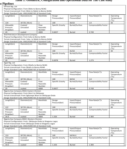
Table 1: Geometric, Configuration and Operational Data for The Case study Gas Pipelines
ElfTotal Nig. Ltd
Physical Configuration: From Obite to Bonny NLNG Terrain transversed: From Obite to Ndele to Bonny NLNG Design Standard Code: ANSI/ASME B31.8 Standard Code
Length(km) Diameter(cm) Manifolds Design
Pressure(bar)
Input/Output Pressure(bar)
Flow Rate(m3/s Operating
Temperature ((0C)
134 36”(91.44cm) 2 100 84/63 1.8 40
Allowable Pressure Drop(bar)
Coated/ Uncoated
Flow Reynolds Number
Specific Gravity Buried/Surface Compressibility Factor
20 coated 4000 0.6657 Buried 0.749
Shell Petroleum Development Company Physical Configuration: From Soku to Bonny NLNG Terrain transversed: From Soku to Ndele to Bonny NLNG Design Standard Code: ANSI/ASME B31.8 Standard Code
Length(km) Diameter(cm) Manifolds Design
Pressure(bar)
Input/Output Pressure(bar)
Flow Rate(m3/s Operating
Temperature ((0C)
116 36”(91.44cm) 1 100 81/63 1.8 40
Allowable Pressure Drop(bar)
Coated/ Uncoated
Flow Reynolds Number
Specific Gravity Buried/Surface Compressibility Factor
20 coated 4000 0.6978 Buried 1.273
Agipl Nig. Ltd
Physical Configuration: From Obiafu to Bonny NLNG Terrain transversed: From Obiafu to Bonny NLNG Design Standard Code: ANSI/ASME B31.8 Standard Code
Length(km) Diameter(cm) Manifolds Design
Pressure(bar)
Input/Output Pressure(bar)
Flow Rate(m3/s Operating
Temperature ((0C)
134 36”(91.44cm) 2 100 84/63 1.8 40
Allowable Pressure Drop(bar)
Coated/ Uncoated
Flow Reynolds Number
Specific Gravity Buried/Surface Compressibility Factor
20 coated 4000 0.6657 Buried 0.749
Nigeria Gas Company (NGC) Eastern Division Physical Configuration: From Warri to Okitipupa
Terrain transversed: From Ogharepe Warri to Okitipupa Ondo Design Standard Code: ANSI/ASME B31.8 Standard Code
Length(km) Diameter(cm) Manifolds Design
Pressure(bar)
Input/Output Pressure(bar)
Flow Rate(m3/s Operating
Temperature ((0C)
122 36”(91.44cm) 2 100 80.6/64 1.8 40
Allowable Pressure Drop(bar)
Coated/ Uncoated
Flow Reynolds Number
Specific Gravity Buried/Surface Compressibility Factor
16.6 coated 4000 1.326 Buried 1.383
Nigeria Gas Company (NGC) Western Division
Physical Configuration: From Okitipupa Ondo to Shagamu Lagos Terrain transversed: From Okitipupa Ondo to Shagamu Lagos Design Standard Code: ANSI/ASME B31.8 Standard Code
Length(km) Diameter(cm) Manifolds Design
Pressure(bar)
Input/Output Pressure(bar)
Flow Rate(m3/s Operating
Temperature ((0C)
153 36”(91.44cm) 2 100 64/44.4 1.8 40
Allowable Pressure Drop(bar)
Coated/ Uncoated
Flow Reynolds Number
Specific Gravity Buried/Surface Compressibility Factor
19.6 coated 4000 1.326 Buried 1.383
(Source :ElfTotal Nig. Ltd, Shell Petroleum Development Company, Agip Nig. Ltd, Nigeria Gas
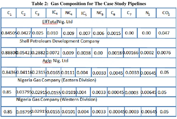
Table 2: Gas Composition for The Case Study Pipelines
Computer Simulation of The Optimization Models
% Computer Programmed for The Determination of The Optimal Flow Parameters (SHELL PAN A)
% Initialization
% Upstream Pressure at OBITE, P1(bar)) P1=84.1;
% Downstream presssure at BONNY, P2(bar) P2=71.0;
% Base pressure, Pbj Pb=1.03;
% Base temperature, Tb Tb=291;
% To calculate average flow pressure, P3 P3=(2/3)*(P1^3-P2^3)/(P1^2-P2^2); disp('P3')
fprintf('%7.3f\n',P3)
% Average flow temperature T=313;
% Line diameter(cm), D D=92.44;
% Elevation above datum, h h=5500;
% Acceleration due gravity, g g=9.8;
% Gsa density GD=73.2404/10^4;
% Pump isentropin efficiency, ni ni=0.85;
% Universal gas constant, R0 R0=8314/10^5;
% Weymouth constant % KW=78.85;
KPA=1.90826;
% Modified Panhandle B constant % KPB=45.03;
% Weymouth exponent, nw % nw=0.5;
% Panhandle A exponent, np n=0.5394;
% Modified Panhandle B exponent, nb % nb=0.51;
% Pipe inlet and exit conditions % Well rounded inlet coeffient, k4 K41=0.04;
% Well rounded exit coefficient, k5 K51=1.0;
% Pump isentropic efficiency, n1 n1=0.95;
% Kinetic energy flux coeffiicient, A2 A2=1.036;
% Area ratio, AR AR=1.0;
% Equivalent length of one globe valves, LEV(m) LEV=350*D;
% Equivalent length of 13 globe valves LEVn=(13*LEV)/1000;
% Equivalent length of one Tee-joint % Flow through run
LET1=20*D; % Flow through branch LET2=60*D;
% Total effective length for 13 Tee-joint LETn=(13*(LET1+LET2))/1000;
% Line lehgth(Km), LL L=131+(LEVn+LETn); for Q=86400:43200:518400 disp('When Q is')
fprintf('%6.2f\n',Q)
% Mean flow velocity, Vm/s) V=(4*Q)/(pi*D^2);
% Pressure ratio, CP CP=2*(P2-P1)/(GD*V^2);
% Average composition of the gas from production line for the month of August 2008(mole fraction) C1A=0.869859;C2A=0.054574;C3A=0.020709;IC4A=0.004517;NC4A=0.006309;IC5A=0.002178;NC5A=0.0 01787;C6A=0.004627;N2A=0.000598;CO2A=0.034843;
% Gas density % GD=73.2924
% Average composition of the gas from production line for the
% month of January 2006(mole fraction)
C1J=0.707881;C2J=0.052663;C3J=0.026519;IC4J=0.005379;NC4J=0.007883;IC5J=0.002642;NC5J=0.002116 ;C6J=0.004207;N2J=0.001332;CO2J=0.028088;
% Specific gravity of the mixture for the month of January, 2006 % GAJ=MGASJ/MAIR;
% Average molecular mass of gaseous mixture(PRODUCTION) in August, 2008
MGASA=(C1A*M11+C2A*M21+C3A*M31+IC4A*M4I1+NC4A*M4N1+IC5A*M5I1+NC5A*M5N1+C6A* M61+N2A*MN21+CO2A*MCO21);
% Specific gravity of the mixture for the month of August, 2008 GAA=MGASA/MAIR;
% Gas density, GD
% GD=(P3*MGASA)/(R0*T); % Gas compressibility factor, Z
Z=((P3*MGASA)/(GD*8314*T))*10; disp(' MGASA GAA Z')
fprintf('%12.6f\n',MGASA,GAA,Z)
% To calculate gas absolute viscosity, GV(Pas--Ns/m2)
% Absolute viscosity of the hydrocarbon components, GVHC, is expressed as:
GVHC=(8.188E-3-6.15E-3*(GAA)+(1.709E-5-2.062E-6*log10(GAA))*(1.8*T+0.27))*1.02247E-5*1.15741E-10;
% *1.15741E-10;
% Absolute viscosity of Nitrogen component
GVN=(9.59E-3+8.48E-3*log10(GAA))*N2A*1.02247E-5*1.15741E-10; % Absolute viscosity of carbon dioxide component
GVC=(6.24E-3+9.08E-3*log10(GAA))*CO2A*1.02247E-5*1.15741E-10; GV=GVHC+GVN+GVC;
disp('GV' )
fprintf('%30.25f\n',GV)
% At the optimal value of Q, dF/dQ=0 % Pump constant, kpp
kpp=(16*GD*(1-n1)/(pi^2*D^4));
% Determination of the optimal flow capacity
K1PA=1.5^(0.0788)*KPA*(1/10^5)^(0.5394)*(Tb/Pb)^(1.0728)*(MAIR/MGASA)^(0.4606)*((GD*(1/10^4)* R0*T*(P1+P2))/(MGASA*(P1^2+P2^2+P1*P2)))^0.0788*((P1+P2)/(T*L))^0.5394*D^2.6182;
K11=((0.0112*GD*L)/(pi^2*D^5))+((8*GD)/(pi^2*D^4))+((8*GD*(K41+A2-1))/(pi^2*D^4))+((8*K51*GD)/(pi^2*D^4));
K12=(1-1/AR^2)*((8*GD)/(pi^2*D^4))+((0.0112*GD*LEVn)/(pi^2*D^5))+((0.0112*GD*LETn)/(pi^2*D^5))+((16*G D*(1-ni))/(pi^2*D^4));
K1=(K11+K12);
K2=0.0014*K1PA^(-1.8539);
K3=((1/(pi^2*D^5))*(0.9256*(GD)^0.68*L*(D*GV)^0.32+0.9256*(GD)^0.68*LEVn*(D*GV)^0.32+0.9256*( GD)^0.68*LETn*(D*GV)^0.32));
%K4=(0.1157*K1PA^(-1.8539)*((D*GV)/(GD*(1/10^4))^0.32); K4=(0.1157*K1PA^(-1.8539)*((D*GV)/(GD^0.32)));
disp('K1PA, K1. K2, K3, K4') fprintf('%20.15f\n',K1PA,K1,K2,K3,K4)
%DF1=((K1PA*GD^0.32*n))*((K1*Q^0.4661+K2*Q^0.32+K3*Q^0.1461+K4+(GD*g*h*Q^(-1.5339)/1000)/(0.0014*(GD*Q)^0.32+0.1157*(D*GV)^0.32))^(n-1));
DF1=((K1PA*GD^0.32*n))*((K1*Q^0.4661+K2*Q^0.32+K3*Q^0.1461+K4+GD*(1/10^3)*g*h*Q^(-1.5339))/(0.0014*(GD*Q)^0.32+0.1157*(D*GV)^0.32))^(n-1);
DF2=(0.0014*(GD*Q)^0.32+0.1157*(D*GV)^0.32);
DF3=(K1*Q^0.4661+K2*Q^0.32+K3*Q^0.1461+K4+GD*(1/10^3)*g*h*Q^(-1.5339))*(4.48*10^(-4)*(GD)^0.32*Q^(-0.68));
DF4=0.4661*K1*Q^(-0.5339)+0.32*K2*Q^(-0.68)+0.1461*K3*Q^(-0.8539)-1.5339*GD*(1/10^3)*g*h*Q^(-2.5339);
DF5=(0.0014*(GD*Q)^(0.32)+0.1157*(D*GV)^(0.32))^(2); disp('DF1,DF2,DF3,DF4,DPF5')
fprintf('%20.15f\n',DF1,DF2,DF3,DF4,DF5) DF=(DF1*((DF2*DF4)+DF3)/DF5);
DPov2=K2*Q^1.8539; DPov3=K3*Q^1.68; DPov4=K4*Q^1.5339; DPov5=GD*g*h/(10^3);
disp('DPov1,DPov2,DPov3,DPov4,DPov5') fprintf('%20.15f\n',DPov1,DPov2,DPov3,DPov4,DPov5) disp('DPov')
fprintf('%20.10f\n',DPov)
% At the optimal flow capacity, DF=0 if DF<=0
disp(' DF Q DPov') fprintf('%20.10f\n',DF,Q,DPov) else
disp('conditions not met') disp(' DF Q DPov') fprintf('%20.10f\n',DF,Q,DPov) end
end
% Computer Programme For The Determination of The Optimal % Maximum orMinimum Values of Flow Capacity and Pressure % Drop((PANHANDLE A)
Q=Oop;
DF1=K1PA*GD^(0.32)*n*(n-1);
DF2=K1*Q^(0.4661)+K2*Q^(0.32)+K2*Q^(0.1461)+K4+GD*g**h*Q^(-1.5339); DF3=0.0014*(GD*Q)^(0.32)+0.1157*(D*GV)^(0.32);
DF4=2.0454E-04*GD^(0.32)*K1*Q^(-0.2139);
DF5=(0.0539*(D*GV)^(0.32)-2.4346E-4*GD*(0.32)*K3)*Q^(-0.5339); DF6=(0.037*(D*GV)^(0.32)*K2-4.48E-4*GD^(0.32))*Q^(-0.68); DF7=0.0169*(D*GV)^(0.32)*K2*Q*(-0.8539);
DF8=0.1775*(D*GV)^(0.32)*GD*g*h*Q^(-2.5339); DF9=-2.5955e-3*GD^(0.32)*GD*g*h*Q^(-2.5339); DF10=DF3^(2);
DF11=K1PA*GD^(0.32)*n; DF12=DF2/df3;
DF13=DF10;
DF14=-4.3751e-5*GD^(0.32)**K1*Q*(-1.2139);
DF15=-(1.4E-4*K3+0.02878*(D*GV)^(0.32))*Q^(-1.5339); DF16=-(0.03516*(D*GV)^(0.32)-3.0464E-4*GD^(0.32)*Q^(-1.68); DF17=-0.0144*(D*GV)^(0.32)*K2*Q^(-1.8539);
DF18=0.005746*GD^(0.32)*GD*g*h*Q^(-3.2139); DF19=0.4498*(D*GV)^(0.32)*GD*g*h*Q^(-3.5339);
DF20=-8.96E-4*GD^(0.32)* (0.0014*(GD*Q)^(0.32)+0.1157*(D*GV)*(0.32)*Q^(-0.68); DF21=8.96E-4*GD^(0.32)*(0.0014*(GD*Q)^(0.32)+0.1157*(D*GV)^(0.32)*Q^(-0.68); DF22=2.0454E-4*GD^(0.32)*K1*Q^(-0.2139);
DF23=(0.0539*(D*GV)*(0.32)-2.4346E-4^GD^(0.32)*K3)*Q^(-0.5339); DF24=0.037*(D*GV)^(0.32)-4.48E-4*GD^(0.32))*Q^(-0.68);
DF25=0.0169*(D*GV)^(0.32)*K2*Q^(-0.8539); DF26=0.1775*(D*GV)^(0.32)*GD*g*h*Q^(-2.5339); DF27=-2.5955E-3*GD^(0.32)*GD*g*h*Q^(-2.5339); DF28=DF3^4;
end
Computer Program for Graphical Presentation of Results % ELF Panhandle B for 36"(0.9144m)
DQop=[-25.413,-24.2427,-8.868,6.608,20.301,41.18,52.9,64.413,77.868,86.991,104.559,118.285]; DD=[-15,-10,-5,5,10,20,25,30,35,40,45,50];
DP1=[-30,-20,-10,10,20,40,50,60,70,80,90,100]; DP2=[-30,-20,-10,10,20,40,50,60,70,80,90,100]; DL=[-15,-10,-5,5,10,20,25,30,35,40,45,50]; %PD=[15.48,12.91,12.34,11.06,10.33,6.56]; plot(DD,DQop,DP1,DQop,DP2,DQop,DL,DQop) %xlabel('P1/P1')
ylabel('Qopt/Qopt')
title('Graph of Change in Optimal Flow Capacity to Optimal flow Capacity and Change in Upstream Pressure to Upstream Pressure ')
%gtext('Upstream/Optimal Line Pressure Drop'),gtext('Downstrean/Optimal Line Pressure Drop
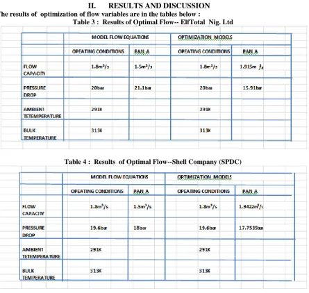
II.
RESULTS AND DISCUSSION
The results of optimization of flow variables are in the tables below :Table 3 : Results of Optimal Flow-- ElfTotal Nig. Ltd
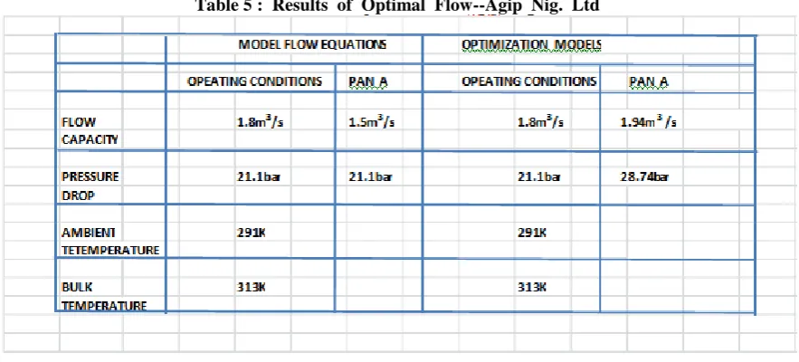
Table 5 : Results of Optimal Flow--Agip Nig. Ltd
Table 6 : Results of Optimal Flow--Nigeria Gas Company (NGC) Eastern Division
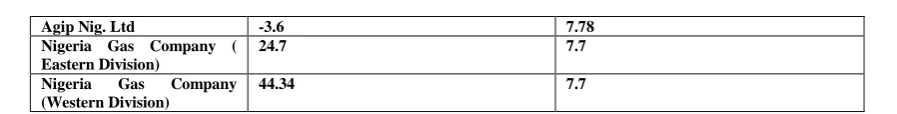
Agip Nig. Ltd -3.6 7.78 Nigeria Gas Company (
Eastern Division)
24.7 7.7
Nigeria Gas Company (Western Division)
44.34 7.7
Table 8 : Reduction in Line Pressure Drop-Increase in Flow Throughput Under Optimized ConditionApparently, there could be a significant improvement on the line pressure drop to the tune of 10 to 45%. Additional flow throughput of 8% above the normal operational level could also be accommodated.
III.
RECOMMENDATION AND CONCLUSION
(i) The optimization scheme clearly confirmed that the present operating conditions of our gas pipelines are truly not optimal. There is therefore urgent need to generate new Design equations incorporating the optimal models for the production of efficient pipelines for future applications. This is to ensure that the operating pipelines and new pipelines networks for gas transmission are not under operated in terms of Pressure-Flow capacity requirements. The design review and analysis would clearlyreduce the cost of design, construction and operations of gas pipelines, associated equipment and facilities. Thus, to plan, set up, operate and execute a gas pipeline at effective cost could be realizable if the optimal pressure-flow capacity requirements are ascertained at the Design and material specification stages. (ii)In-depth research work is recommended in the area of theoretical, practical and economic consideration of flow compressibility effects as well as hydration problems in sub-cooled under water offshore pipelines. Adequate knowledge of compressibility effects on pressure drop and pressure gradient will go a long way in ascertaining the operating pressure-temperature characteristics of pipelines so as to correlate the operating measured conditions.
(iii) Critical review of as-installed physical, geometric and flow features of gas pipelines for more exact evaluation of losses in fluid energy. If the factors influencing the loss of fluid energy are thoroughly evaluated, the required overall pressure drop in a gas pipeline could be closely specified. This will off-set the problem of underrating or overrating the Pressure–Flow capacity requirements for gas pipelines. This would also aid the sizing of compressors, pumps, valves, fittings and metering devices.
(iv) This optimization and sensitivity analysis is limited to single phase flow of gas. Future research is envisaged to also address optimization models for two phase flow of gas in gas transmission pipelines[ PhD Yhesis ].
Conclusion
Gas Pipeline flow optimization models developed by the researcher for single phase flow of gas have simulated by computationapproach. The simulation results clearly confirmed that there could drastic reduction in pressure drop for the optimized gas pipelines. Additional throughput of about 10% could be accommodated over the normal operational level. Analysis of the optimization results clearly confirmed that operating optimally would have significant impact in reducing the cost of investment and operation of as installed gas pipelines, even the future generation of gas pipelines to be in Nigerian terrain.
REFERENCES
[1]. Adeyanju, O. A. and Oyekunle, L. O. (2012): “Optimization of Natural Gas Transmission in Pipeline”, Oil and Gas Journal, Vol.
69, No 51.
[2]. Shadrack, MathewUzoma&Abam, D. P. S., “Flow Optimization Models In Gaspipelines (Modified Panhandle-B Equation As Base
Equation)”, Journalof Scienceand Technology Research, Vol. 6, No. 1, Pp 31-41, April 2013.
[3]. Shadrack, Mathew Uzoma&Abam, D. P. S., “Flow Optimization Models In Gas pipelines(Weymouth Equation As Base Equation)”,
African Scienceand Technology Journal Siren Research Centrefor African Universities, Vol. 6, No. 1, Pp 109-123, April 2013.
[4]. Abam, D. P. S. &Shadrack, MathewUzoma, “Flow Optimization Models In Gas pipelines(Panhandle-A Equation As Base
Equation)”, Journalof Scienceand Technology Research, Vol. 6, No. 3, Pp 1-16, December, 2013.
[5]. Shadrack, Mathew Uzoma, “Flow Optimization In Natural Gas Pipeline”, PhD Thesis,April, 2016, Department of Mechanical
Engineering,University of Port Harcourt, Port Harcourt, Rivers State, Nigeria.
[6]. Guo, B.; Ghalambor, A. and Xu, C. (2005): “A Systematic Approach to Producing Liquid Loading in Gas Wells”, paper
SPE94081, presented at the SPE production operations symposium, Oklahoma city, April 17-19.
[7]. Fox and McDonald (1981): Introduction to fluid Mechanics, 2nd edition, John Wiley and Sons Inc. New York.
[8]. Anderson, Allen (1993): “Alfred Rowe and the RO Ranch”, Panhandle Plain Historical Review; Pp 24-52.