An Α-Series Process Optimal Replacement Problem For A Shock Model With Two-Type Failures

Volume 8, Issue 3 (August 2013), PP. 01-06

An Α-Series Process Optimal Replacement Problem For A

Shock Model With Two-Type Failures

M.Sreedhar

1

, Dr.R.Bhuvana Vijaya

2

, Dr. B. Venkata Ramudu

3 1

Dept. of Mathematics, JNTUA College of Engineering,Anantapur-515 002. A.P (India) . 2

Assistant Professor & Head, Dept. of Mathematics, JNTUA College of Engineering,Anantapur-515 002. A.P (India) .

3

Assistant Professor, Dept. of Statistics, SSBN Degree College (Autonomous)Anantapur-515 002, A.P (India).

Abstract:- This paper studies a shock model for a repairable system with two-type failures by assuming that two kinds of shocks in a sequence of random shocks will make the system failed, one based on the inter-arrival time between two consecutive shocks less than a given positive value and the other based on the shock magnitude of single shock more than a given positive value. Further it is assumed that the system after repair is not ‘as good as new’, but the consecutive repair times of the system form a stochastic increasing α-series process. Under these assumptions, we determine an explicit expression for the average cost rate and an optimal placement policy N* based on the number of failure of the system is determined such that the long-run average cost per unit time is minimized. The explicit expression of long-run average cost per unit time is derived, and the corresponding optimal replacement policy can be determined analytically or numerically. Finally, a numerical example is given.

Keywords:- Replacement policy, α-series process, renewal reward theorem, Average cost rate, MTTF.

I. INTRODUCTION

The shock model mainly used to study the external causes such as the environmental factor which may influence system reliability. For example, a precision instrument and meter installed in a power workshop may be affected by some random shocks due to the operation of other instruments, such as lathes or electrical machineries. Esary at al. [4] examined the theory of Poisson shock model. Later on, Barlow and Proschan [2] studied this problem in their monograph. Ross [14] developed a generalized Poisson shock model. Shantikumar and Sumita [16] extended Poisson shock to general shock, and studied a such shock model in which a system fails when the shock magnitude of single shock outstrips a given positive value. At the same time, Feldman [5], Zuckerman [24], Gottlieb [7] and Abdel-Hammed [1] determined respectively the optimal replacement policy for the different shock models. Li et al. [12] presented a new shock model named δ-shock model. Wang and Zhang [19] not only considered some reliability indices of the δ-shock model, but also studied geometric process repair model and its optimal replacement policy.

For a deteriorating system, a more reasonable repair model is the geometric process repair model first proposed by Lam [8, 9]. Under this model, Lam considered two kinds of replacement policy, one based on the working age T of the system and the other based on the failure number N of the system. It assumed that the consecutive working times of the system form a decreasing geometric process while the consecutive repair times of the system form a increasing geometric process and the system after repair is not ‘as good as new’ state. Under these assumptions an explicit expressions for the long-run average cost per unit time under these two kinds of policy are respectively derived, and the corresponding optimal replacement policies T* and N* are found analytically or numerically. Because the geometric process is a special monotone process, Stadje and Zuckerman [17] introduced a general monotone process repair model to generalize Lam’s work. Zhang [21] generalized Lam’s work by a bivariate replacement policy (T, N) under which the system is replaced at the working age T or at the time of the Nth failure, whichever occurs first. Later for improving the system reliability and its availability, Zhang [22] utilized the geometric process repair model to a two-component cold standby system with one repairman. It assumed that each component after repair is not ‘as good as new’. Under these assumptions, a replacement policy N based on the number of repair of component 1 is considered. He determined the optimal replacement policy N* such that the long-run expected reward per unit time s maximized. Many research works have been done by Zhang [23], Stadje and Zuckerman [18], Finkelstein [6], Wang and Zhang [19], Lam and Zhang [10, 11].

process. Under these assumptions a replacement policy N based on the number of failures of the system is determined such that the long-run average cost rate is minimized. Braun et.al [3] examined the increasing geometric process grows at most logarithmically in time, while the decreasing geometric process is almost certain to have a time of explosion. The α-series process grows either as a polynomial or exponential in time. It also noted that the geometric process doesn’t satisfy a central limit theorem, while the α-series process does.

Based on this understanding, this paper generalize Wang and Zhang [20] shock model for a repairable system with two-type failures model by the α -series process model. It is assumed that two kinds of shock in a sequence of random shocks will make the system failed, one based on the inter arrival time between two consecutive shocks less than a given positive value δ (i.e. so-called ‘δ-shock model’) and the other based on the shock magnitude of single shock more than a given positive value δ (i.e. so-called ‘δ- shock model’). Assume further that the system after repair is ‘as good as new’ while the consecutive up times of the system will become longer and longer. Under these assumptions, by using the α-series process repair model, a replacement policy N based on the number of failure of the system is studied. The problem is to obtain an optimal replacement policy N* such that the long-run average cost per unit time is minimized. An explicit expression of the long-run average cost per unit time is derived, and hence an optimal policy N* can be determined analytically or numerically. Finally, a numerical example is given.

For understanding the model, we considered the definition (see Braun [3]) of α- series process as follows.

Definition 1:

Given two random variables X and Y, if P(X>t) > P(Y>t) for all real t, then X is called stochastically larger than Y or Y is stochastically less than X. This is denoted by X >st Y or Y <st X respectively.

Definition 2:

Assume that {Xk, k=1,2,….}, is a sequence of independent non-negative random variables. If the distribution function of Xk is

F

k

(

t

)

F

(

k

t

)





for some α > 0 and all k=1, 2, 3… then {Xk, k=1, 2…} is called an α-series process, α is called exponent of the process.

Obviously:

if α>0, then {Xk, k=1,2,….} is stochastically decreasing, i.e, Xk >st Xk+1 , k=1,2,…; if α<0, then {Xk, n=1,2,….} is stochastically increasing, i.e., Xk <st Xk+1 , k=1,2,; if α=0, then the



series process becomes a renewal process.

II. THE Δ-SHOCK MODEL

In most of the situations where random shock occurs, it can be observed that the system reliability is decreasing. In ordered to raise the system reliability, we consider two kinds of random shock such that the system is failed. Let Tk and Dk denote respectively the time interval between (k-1)th shock and kth shock, and the magnitude of kth shock.

Let δ and γ be two positive in the system. The system will fail as soon as Tk< δ appears, k=1, 2, . . . and the system failure caused by Tk< δ is called the first type failure. In fact, it is a _-shock model considered by Wang and Zhang (2001). Similarly, the system will fail as soon as Dk>γ, k=1, 2, . . . appears and the system failure caused by Dk>γ is called the second type failure. In fact, it is a shock model considered by Shanthikumar and Sumita (1983). Remember that the system will fail as soon as both Tk<δ and Dk>γ appears k=1, 2, . . . . Thus, we may as well call the system failure the third type failure. In other words, two-type failures will cause three cases of the system failure. It is a more extensive shock model in which we not only consider the magnitude of single shock but also the time interval of consecutive two shocks to the effect of the system.

Let S1, S2, . . . be shock arrival time when the system is working, and assume that

{Tk, k=1, 2, . . .} and {Dk, k=1, 2, . . . } are respectively a sequence of i.i.d. non-negative random variables. Clearly,

..

…

1,2,

=

k

,

T

+

..

…

…

+

T

+

T

=

S

k 1 2 k (2.1)

Let X be the working time before the system first fails, then

.

T

+

..

…

…

+

T

+

T

_{1 2 M}



X

(2.2) Where, M is shock number of times at the system failure, and it is a random variable. Now, we give out

some results of the system under shock model with two-type failure.

Theorem 1: Assume that {(Tk, Dk), k = 1, 2, . . .} forms a correlated renewal sequence pair with joint distribution function

 

x

,

y

P



T

x

,

D

y



,

and H(t) is the distribution function of X, then the Laplace transform of H(t) is given by

(2.3)

parameters positive

given two

are and

y x dF e

s F dx x F e s

F

where _T ( ) sx _T( ) , ( ,



) sx _T( , ),





0 *

0 *





 



 _



[See G. J. Wang & Y. L. Zhang (2005)]

Thus, we can get the system reliability R(t) =



H

(t) . From Theorem 1 we have

P00 = P(T≥δ, D≤



), (2.4)

P10 = P(T<δ, D≤



), (2.5)

P01 = P(T≥δ, D>



), (2.6)

and

P11 = p(T<δ, D>



), (2.7)

denote respectively the probabilities that neither the first type failure nor the second type failure happens, only the first type failure happens, only the second type failure happens and both the two-type failures happen in the system. Clearly, p00+p10+p01+p11=1.

Theorem 2: Under the condition of Theorem 1 given by G. J. Wang & Y. L. Zhang [20] , the mean working time before the system fails is given by:

. 1 ] ... [

00 2

1

p ET T

T T E

EX     M  _

(2.8) We make the following assumptions about the repairable system for random shock with two-type failures.

1. In the initial stage, the system is new. The system will be repaired as soon as it failed. The system will be replaced some time by a new and identical one, and the replacement time is negligible.

2. Assume that the system after repair is ‘as good as new’ while the consecutive repair times of the system form a stochastic increasing α- series process. The time interval between the completion of the (k-1)-th repair and the completion of the k-th repair on the system is called the k-th cycle of the system, k=1, 2, . . . .

3. Let

X

_k(i) and

Y

_k(i) be respectively the working time and the repair time of the system incurred by i-th type failure in the k-th cycle, i=1, 2, 3; k=1, 2, . . . . and both the times form a decreasing α- series process and increasing α- series process respectively.

4. Let {

X

_k(i), k=1, 2, . . . } is a sequence of the i.i.d. non-negative random variables distributed

according to an exponential failure law with distribution function

F

(

k



t

)

, while the distribution of

) (i k

Y

is assumed to be

G

(

k



t

)

, and the assume that ET1=λ and E

) (i k

Y

=μi , where t≥0, 0<β<1, λ>0, μi >0; i=1, 2, 3; k=1, 2, . . . .

5. Assume that

X

_k(i),

Y

_k(i), i=1, 2, 3; k=1, 2, . . . are independent.

6. Let

ET





be the average working time.

7. The replacement policy N based on the failure number of the system is used.

8. Assume that the repair cost incurred by i-th type failure of the system per unit time is

c

r(i) , i=1, 2, 3,

the working reward of the system per unit time is cw, and the replacement cost of the system is C.

III. LONG-RUN AVERAGE COST RATE UNDER POLICY N

Now, our problem is to determine an optimal replacement policy N such that the long-run average cost per unit time is minimized.

between two consecutive replacements is a renewal cycle. Then according to the renewal reward theorem (see, for example, Ross [13-15]), we have

.

exp

cos

exp

)

(

cycle

a

of

length

ected

the

cycle

a

in

incurred

t

ected

the

N

C



(3.1)

Where the length of the renewal cycle is given by









1

) 3 ( 2 ) 3 ( 2 ) 2 ( 2 ) 2 ( 2 ) 1 ( 2 ) 1 ( 2 2 ) 3 ( 1 ) 3 ( 1 ) 2 ( 1 ) 2 ( 1 ) 1 ( 1 ) 1 ( 1

1

















...







X

Y

I

Y

I

Y

I

X

Y

I

Y

I

Y

I

X

_N

W



(3)1



.

) 3 ( 1 ) 2 ( 1 ) 2 ( 1 ) 1 ( 1 ) 1 (

1 N N N N N N

N

I

Y

I

Y

I

X

Y









_{     }

(3.2)

To evaluate EW, we only need to calculate the following results by using the property of the conditional expectation



(

|

)



(

1

)

(

)

)

(

Y

k(1)

I

k(1)

E

E

Y

k(1)

I

k(1)

I

k(1)

P

I

k(1)

E

Y

k(1)

E







(3.3)



(

|

)



(

1

)

(

)

)

(

(2) (2) (2) (2) (2) (2) (2)

k k k k k k

k

I

E

E

Y

I

I

P

I

E

Y

Y

E







(3.4)



(

|

)



(

1

)

(

)

)

(

Y

k(3)

I

k(3)

E

E

Y

k(3)

I

k(3)

I

k(3)

P

I

k(3)

E

Y

k(3)

E







(3.5) Let qi, i=1, 2, 3 be the probability of the ith type failure when failure happen, then

00 10 ) 1 ( 1 ) 1 ( 1 ) 1 ( ) ( P P I P q I

E k   k   _{ (3.6)}

00 01 ) 2 ( 2 ) 2 ( 1 ) 1 ( ) ( P P I P q

E k   k   _{ (3.7)}

. 1 ) 1 ( ) ( 00 11 ) 3 ( 3 ) 3 ( P P I P q I

E k   k   _

(3.8)

Clearly, q1+ q2 +q3 =1 ; and

00 10 1 1 1 ) 1 ( ) 1 ( 1 . ) ( 1 1 _P P k q k I Y

E k k     _

  (3.9)





00 01 2 2 2 ) 2 ( ) 2 ( 1 . 2 2 _P P k q k I Y E _{k k}

 

 _ _{ (3.10)}





00 11 3 3 3 ) 3 ( ) 3 ( 1 . 3 3 _P P k q k I Y

E k k     _

 

(3.11)

According to the assumption (6) of the model and using equations (3.9) to (3.11), the expected length of a renewal cycle is







     









1 1 3 3 1 1 2 2 1 1 1

1 _{1 2 3}

1

1

1

N k N k N k

k

q

k

q

k

q

NEX

EW



_



_



_

(3.12)







              1 1 00 11 3 1 1 00 01 2 1 1 00 10 1 00 3 2 1 1 1 1 1 1 1 1 N k N k N

k p k

p k p p k p p p N        (3.13)

According to equations (3.1) and (3.2), we have

 

 

 

EW NEX c C Y E q c Y E q c Y E q c w N k k r N k k r N k k

r











 

      1 1 ) 3 ( 3 3 ) 3 ( 1 1 ) 2 ( 2 2 ) 2 ( 1 1 ) 1 ( 1 1 ) 1 ( = C(N)   

According to equations (3.3) and (3.13), we have

Where









1

1

1 ₁

1

N

k

k

l

_ ,









1

1 2

2

1

N

k

k

l

_{ ,}









1 1

3 ₃

1

N

k

k

l

_

In the next section, numerical results are provided to highlight the obtained theoretical results.

IV. NUMERICAL RESULTS AND CONCLUSIONS:

For the given hypothetical values of the parameters μ1, μ2, μ3, λ, Cr(1) , Cr(2), Cr(3), q1, q2, q3 , β1, β2, β3, C ,and Cw we determine the long run average cost per unit time from the equation (9) as follows:

Where μ1=20,μ2=30,μ3=50,, λ=80, Cr(1) =3, Cr(2)=5, Cr(3)=10, q1=0.45, q2=0.4, q3=0.15, β1=-0.65, β2=-0.75, β3 =-0.85, C=7000 ,and Cw=50.

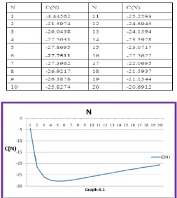
Table 4.1: Values of the Long-Run Average Cost Rate Under Policy N.

V. CONCLUSIONS

1.From the table 4.1 and graph 4.1, it is examined that the long-run average cost per unit time is minimum when the number of failure of the system reaches 6.i.e., C(6)=-27.7511 at β1=-0.65, β2=-0.75 , β3 =-0.85.Thus the system should be replaced at the time of 6th failure.

2.The decreasing



-series process may be more appropriate for modeling system working times while the increasing geometric process is more suitable for modeling repair times of the system. It assumed that the system after repair is not ‘as good as new’ and also the successive working times form a decreasing



-series process, the successive repair time’s form an increasing α- -series process and both the processes are exposing to exponential failure law. Under these assumptions we study an optimal replacement policy N in which we replace the system when the number of failures reaches N. We determine an optimal repair replacement policy N* such that the long run average cost per unit time is minimized.

3.If the repair man is familiar with the repair the successive repair times stochastically non-increasing and the successive working times are stochastically non-decreasing. Thus this model can also be applied for an improved system exposing to Weibull failure law.

REFERENCES

[1] M. Abdel-Hameed, ‘Optimum replacement of systems subject to shocks’, Journal of Applied Probability, 1986, 23, pp. 107–114.

[3] Braun W.J, Li Wei and Zhao Y.Q, ‘Properties of the geometric and related process’, Naval Research Logistics, Vol.52, pp.607-617, 2005.

[4] J.D. Esary, A.W. Marshall and F. Proschan, ‘Shock models and wear processes’, Annals of Probability, 1973, 1, pp. 627–650.

[5] R.M. Feldman, ‘Optimal replacement with semi-Markov shock models’, Journal of Applied Probability, 1976, 13, pp. 108–117.

[6] M.S. Finkelstein, ‘A scale model of general repair’, Microelectronic Reliability, 1993, 33, pp. 41–44. [7] G. Gottlieb, ‘Optimal replacement for shock models with general failure rate’, Operations Research,

1982, 30, pp. 82–92.

[8] Y. Lam, ‘Geometric processes and replacement problem’, Acta Mathematicae Applicatae Sinica, 1988a, 4, pp. 366–377.

[9] Y. Lam, ‘A note on the optimal replacement problem’, Advances in Applied Probability, 1988b, 20, pp. 479–782.

[10] Y. Lam and Y.L. Zhang, ‘Analysis of a two-component series system with a geometric process model’, Naval Research Logistics, 1996a, 43, pp. 491–502.

[11] Y. Lam and Y.L. Zhang, ‘Analysis of a parallel system with two different units’, Acta Math. Appl. Sin., 1996b, 12, pp. 408–417.

[12] Z.H. Li, B.S. Huang and G.J. Wang, ‘Life distribution and statistical property of shock model with a shock source’, Journal of Lanzhou University, 1999, 35, pp. 1–8.

[13] S.M. Ross, Applied Probability Models with Optimization Applications, San Francisco: Holden-Day, 1970.

[14] S.M. Ross, ‘Generalized poisson shock models’, Annals of Probability, 1981, 9, pp. 896–898. [15] S.M. Ross, Stochastic Processes, 2nd edition, New York: Wiley, 1996.

[16] J.G. Shanthikumar and U. Sumita, ‘General shock model associated with correlated renewal sequences’, Journal of Applied Probability, 1983, 20, pp. 600–614.

[17] W. Stadje and D. Zuckerman, ‘Optimal strategies for some repair replacement models’, Advances in Applied Probability, 1990, 22, pp. 641–656.

[18] W. Stadje and D. Zuckerman, ‘Optimal repair policies with general degree of repair in two maintenance models’, Operations Research Letters, 1992, 11, pp. 77–80.

[19] G.J. Wang and Y.L. Zhang, ‘δ-shock model and its optimal replacement policy’, Journal of Southeast University, 2001, 31, pp. 121–124.

[20] G.J. Wang and Y.L. Zhang, A-shock model with type failures and optimal replacement policy’, International Journal of Systems Science, 2005, 36, pp. 209–214.

[21] Y.L. Zhang, ‘A bivariate optimal replacement policy for a repairable system’, Journal of Applied Probability, 1994, 31, pp. 1123–1127.

[22] Y.L. Zhang, ‘An optimal geometric process model for a cold standby repairable system’, Reliability Engineering and Systems Safety, 1999, 63, pp. 107–110.

[23] Y.L. Zhang, ‘A geometric process repair model with good-as-new preventive repair’, IEEE Transactions on Reliability, 2002, R-51, pp. 223–228.