e-ISSN: 2278-7461, p-ISSN: 2319-6491
Volume 5, Issue 7 [Aug. 2016] PP: 38-47
Collocation Method for Ninth order Boundary Value
Problems Using Quintic B-Splines
S. M. Reddy
Department of Science and Humanities, Sreenidhi Institute of Science and Technology,Hyderabd-India-501 301
Abstract
:
A finite element method involving collocation method with septic B-splines as basis functions has been developed to solve ninth order boundary value problems. The ninth, eight and seventh order derivatives for the dependent variable is approximated by the finite differences. The basis functions are redefined into a new set of basis functions which in number match with the number of collocated points selected in the space variable domain. The proposed method is tested on two linear and one nonlinear boundary value problems. The solution to a nonlinear problem has been obtained as the limit of a sequence of solutions of linear problems generated by the quasilinearization technique. Numerical results obtained by the present method are in good agreement with the exact solutions available in the literature.Keywords: Collocation method, Septic B-spline, Ninth order boundary value problem, Absolute error.
I.
INTRODUCTION
In this paper, we consider a general ninth order boundary value problem
( 9 ) ( 8 ) ( 7 ) ( 6 ) ( 5 )
( 4
0 1 2 3 4
5 6 7 8 9
)
( ) ( ) ( ) ( ) ( ) ( ) ( ) ( ) ( ) ( )
( ) ( ) ( ) ( ) ( ) ( ) ( ) ( ) ( ) ( ) ( ) ,
a x y x a x y x a x y x a x y x a x y x
a x y x a x y x a x y x a x y x a x y x b x c x d
(1)
subject to boundary conditions
0 0 1 1 2 2 3
( 4 )
3 4
,
( ) , ( ) , ( ) , ( ) , ( ) ( ) , ( ) , ( ) ,
( )
y c A y d C y c A y d C y c A y d C y c A y d C
y c A
(2)
where A0, A1, A2, A3, A4,C0, C1, C2, C3, are finite real constants and a0(x), a1(x), a2(x), a3(x), a4(x), a5(x), a6(x), a7(x), a8(x), a9(x) and b(x) are all continuous functions defined on the interval [c, d].
The ninth-order boundary value problems are known to arise in the study of astrophysics, hydrodynamic and hydro magnetic stability [5]. A class of characteristic-value problems of higher order (as higher as twenty four) is known to arise in hydrodynamic and hydromagnetic stability [5]. The existence and uniqueness of the solution for these types of problems have been discussed in Agarwal [2]. Finding the analytical solutions of such type of boundary value in general is not possible. Over the years, many researchers have worked on ninth-order boundary value problems by using different methods for numerical solutions. Chawla and Katti [6] developed a finite difference scheme for the solution of a special case of nonlinear higher order two point boundary value problems. Wazwaz [16] developed the solution of a special type of higher order boundary value problems by using the modified Adomian decomposition method. Hassan and Erturk [1] provided solution of different types of linear and nonlinear higher order boundary value problems by using Differential transformation method. Tauseef and Ahmet [14] presented the solution of ninth and tenth order boundary value problems by using homotopy perturbation method without any discretization, linearization or restrictive assumptions. Tauseef and Ahmet [15] developed modified variational method for solving ninth and tenth order boundary value problems introducing He’s polynomials in the correction functional. Jafar and Shirin [8] presented homotopy perturbation method for solving the boundary value problems of higher order by reformulating them as an equivalent system of integral equations. Tawfiq and Yassien [9] developed semi-analytic technique for the solution of higher order boundary value problems using two-point oscillatory interpolation to construct polynomial solution. Hossain and Islam [3] presented the Galerkin method with Legendre polynomials as basis functions for the solution of odd higher order boundary value problems. Samir [12] developed spectral collocation method for the solution of mth order boundary value problems with help of Tchebyshev polynomials by converting the given differential equation into a system of first order boundary value problems. So far, ninth order boundary value problems have not been solved by using collocation method with septic B-splines as basis functions.
the collocation method with septic B-splines as basis functions has been presented and in section V, solution procedure to find the nodal parameters is presented. In section VI, numerical examples of both linear and non-linear boundary value problems are presented. The solution to a nonnon-linear problem has been obtained as the limit of a sequence of solution of linear problems generated by the quasilinearization technique [4]. Finally, the last section is dealt with conclusions of the paper.
II.
JUSTIFICATION
FOR
USING
COLLOCATION
METHOD
In finite element method (FEM) the approximate solution can be written as a linear combination of basis functions which constitute a basis for the approximation space under consideration. FEM involves variational methods like Ritzs approach, Galerkins approach, least squares method and collocation method etc. The collocation method seeks an approximate solution by requiring the residual of the differential equation to be identically zero at N selected points in the given space variable domain where N is the number of basis functions in the basis [10]. That means, to get an accurate solution by the collocation method one needs a set of basis functions which in number match with the number of collocation points selected in the given space variable domain. Further, the collocation method is the easiest to implement among the variational methods of FEM. When a differential equation is approximated by mth order B-splines, it yields (m + 1)th order accurate results [11]. Hence this motivated us to solve a ninth order boundary value problem of type (1)-(2) by collocation method with septic B-splines as basis functions.
III.
DEFINITION
OF
SEPTIC
B-SPLINES
The septic B-splines are defined in [7, 11, 13]. The existence of septic spline interpolate s(x) to a function in a closed interval [c, d] for spaced knots (need not be evenly spaced) of a partition c = x0 < x1 <…< xn-1 < xn= d
is established by constructing it. The construction of s(x) is done with the help of the septic B-splines. Introduce fourteen additional knots x-7, x-6, x-5, x-4, x-3, x-2, x-1, xn+1, xn+2, xn+3, xn+4, xn+5, xn+6 and xn+7 in such a way that x-7<x-6<x-5<x-4<x-3<x-2<x-1<x0 and xn<xn+1<xn+2<xn+3<xn+4< xn+5< xn+6< xn+7.
Now the septic B-splines Bi(x)'s are defined by
7 4
4 4
4
( )
, [ , ]
( ) ( )
0 , i
r
i i
r i
i r
x x
x x x
B x x
o t h e r w i s e
where
7
7 ( ) ,
( )
0 ,
r r
r
r
x x if x x
x x
if x x
and
4
4
( ) ( )
i
r r i
x x x
where {B-3(x), B-2(x), B-1(x), B0(x), B1(x),…,Bn(x), Bn+1(x), Bn+2(x), Bn+3(x)} forms a basis for the spaces7() of septic polynomial splines. Schoenberg [13] has proved that septic B-splines are the unique nonzero splines of smallest compact support with the knots at
x-7<x-6<x-5<x-4<x-3<x-2<x-1<x0<x1<…<xn-1<xn<xn+1<xn+2<xn+3<xn+4<xn+5<xn+6<xn+7.
IV.
DESCRIPTION
OF
THE
METHOD
To solve the boundary value problem (1) subject to boundary conditions (2) by the collocation method with septic B-splines as basis functions, we define the approximation for y x( ) as
3
3
( ) ( )
n
j j j
y x B x
Where j's are the nodal parameters to be determined and Bj( ) 'x s are septic B-spline basis functions. In the
present method, the mesh points
2 2, 3, ...., n , n 1
x x x x are selected as the collocation points. In collocation method,
the number of basis functions in the approximation should match with the number of collocation points [6]. Here the number of basis functions in the approximation (3) is n+7, where as the number of selected collocation points is n-2. So, there is a need to redefine the basis functions into a new set of basis functions which in number match with the number of selected collocation points. The procedure for redefining the basis functions is as follows:
Using the definition of septic B-splines, the Dirichlet, Neumann, second order derivatives boundary conditions, third order derivative boundary conditions and fourth order derivative boundary condition of (2), we get the approximate solution at the boundary points as
0 0 0
3 3
( ) ( ) j j( )
j
y c y x
B x A
(4)3
0 3
( ) ( ) ( )
n
n j j n
j n
y d y x
B x C
(5)0 0 1
3 3
( )
(
)
j j(
)
j
y
c
y
x
B
x
A
(6)3
1 3
( ) ( ) ( )
n
n j j n
j n
y d y x
B x C
(7)0 0 2
3
3
( ) ( ) j j( )
j
y c y x
B x A
(8)2 3
3
(
)
(
)
(
)
n
n j j
j n
n
y
d
y
x
B
x
C
(9)3
3
0 0
3
( ) ( ) j j ( )
j
y c y x
B x A
(10)3
3 3
(
)
(
)
(
)
n
j j
j n
n n
y
d
y
x
B
x
C
(11)( 4 ) ( 4 ) ( 4 )
0 0
3 3
4
( ) ( ) j j ( )
j
y c y x
B x A
(12)Eliminating 3,2,1, 0, 1, n, n1,n2 and
n3 from the equations (3) to (12), we get the approximation for y(x) as1
2
( )
( )
( )
n
j j
j
y x
w x
T
x
(13)Where
4
( 4 ) 4
( 1
1
0 4 )
0
(
( ) ( ) ( )
( )
)
A
w x w x S
S x
w
x x
3 3 0 3 3 0 0 4 3 0 ( ) ( ) ( ) ( ) ( ) ( ) ( ) ( ) n n n n A
w x w x R x R x
x x
w x C w x
R R 2 2 2
0 2 2
1
1 0 1
3 1
(
( ) ( ) ( ) ( )
( ) ( )
) ( n)
n n n
w x w x
Q Q
A C
w x w x Q x Q x
x x
1 1 0 1 1
2 2 2 1 2 0 2 ( ) ( ) ( ) ( ) ( ) ( ) ( ) ( ) n n n n A C
w x w x w x P x w x P x
x P x
P
0 0
1 3 3
3 0 3
( ) ( ) ( )
( ) n ( n) n
A C
w x B x B x
B x B x
( 4 ) 0
1 ( 4 )
1 0
( )
( ) ( ) , 2 , 3
( ) ( )
( ) , 4 , 5 , ..., 1
j j
j
j
S x
S x S x j
T x S x
S x j n
(14) 0 0 0 0 ( )
( ) ( ) , 1, 2 , 3
( )
( ) ( ) , 4 , 5 , ..., 4
( )
( ) ( ) , 3 , 2 , 1
( )
j j
j j
j n
j n n
n n
R x
R x R x j
R x
S x R x j n
R x
R x R x j n n n
R x 0 1 1 0 1 1 ( )
( ) ( ) , 0 , 1, 2 , 3
( )
( ) ( ) , 4 , 5 , ..., 4
( )
( ) ( ) , 3 , 2 , 1,
( ) j j j j j n j n n n Q x
Q x Q x j
Q x
R x Q x j n
Q x
Q x Q x j n n n n
Q x 0 2 2 0 2 2 ( )
( ) ( ) , 1, 0 , 1, 2 , 3
( )
( ) ( ) , 4 , 5 , ..., 4
( )
( ) ( ) , 3 , 2 , 1, , 1
( ) j j j j j n j n n n P x
P x P x j
P x
Q x P x j n
P x
P x P x j n n n n n
P x 0 3 3 0 3 3 ( )
( ) ( ) , 2 , 1, 0 , 1, 2 , 3
( )
( ) ( ) , 4 , 5 , ..., 4
( )
( ) ( ) , 3 , 2 , 1, , 1, 2
( ) j j j j j n j n n n B x
B x B x j
B x
P x B x j n
B x
B x B x j n n n n n n
Now the new basis functions for the approximation y(x) are {Tj(x), j=2, 3,…, n-1} and they are in
number match with the number of selected collocated points. Since the approximation for y(x) in (13) is a septic approximation, let us approximate y(7) , y(8) and y(9) at the selected collocation points with finite differences as
( 6 ) ( 6 )
( 7 ) 1 1
f o r
2 , 3, ...,
1
2
i i
i
y
y
y
i
n
h
(15)( 7 ) ( 7 ) ( 7 )
( 8 ) 1 1
2
2
f o r 2 , 3, ...., 1
i i i i
y y y
y i n
h
(16)
( 6 ) ( 6 ) ( 6 ) ( 6 )
( 7 ) 2 1 1 2
3
2 2
f o r 2 , 3, ...., 2 2
i i i i i
y y y y
y i n
h
(17)
( 6 ) ( 6 ) ( 6 ) ( 6 )
( 9 ) 1 2 3
3
3 3
f o r 1
i i i i
i
y y y y
y i n
h
(18)
where
1
2
( ) ( ) ( )
n
i i i j j i j
y y x w x T x
(19)Now applying the collocation method to (1), we get
( 9 ) ( 8 ) ( 7 ) ( 6 ) ( 5 ) ( 4 )
0 2 3 4 5
6 7 8
1
9
( ) ( ) ( ) ( ) ( ) ( )
( ) ( ) ( ) ( ) ( ) f o r 2 , 3 , , 1 .
i i i i i i i i i i i i
i i i i i i i i i
a x y a x y a x y a x y a x y a x y
a x y a x y a x y a x y b x i n
(20)
Substituting (15) to (19) in (20), we get
1 1 1
( 6 ) ( 6 ) ( 6 ) ( 6 ) ( 6 ) ( 6 ) ( 6 )
2 2 1 1 1 1 2
2 2 2
0
3 1
( 6 ) 2 2
1
( 6 ) ( 6 ) ( 6 )
1
1 1
2
2
( ) ( ) 2 ( ) 2 ( ) 2 ( ) 2 ( ) ( )
( ) 2
( )
( )
( ) ( ) 2 (
n n n
i j j i i j j i i j j i i
j j j
i n
j j i
j
n i
i j j i i
j
w x S x w x S x w x S x w x
a x
h
S x
a x
w x T x w x
h
1 ( 6 ) ( 6 ) 1 ( 6 )1 1
2 2
1 1
( 6 ) ( 6 ) ( 6 ) ( 6 )
2
1 1 1 1
2 2
1
( 6 ) ( 6 ) ( 5 ) ( 5 )
3 4
2
) 2 ( ) ( ) ( )
( )
( ) ( ) ( ) ( )
2
( ) ( ) ( ) ( ) ( )
n n
j j i i j j i
j j
n n
i
i j j i i j j i
j j
n
i i j j i i i j j
j j
T x w x T x
a x
w x T x w x T x
h
a x w x T x a x w x T
1 ( 4 ) 1 ( 4 )5 2 2 1 1 6 7 2 2 1 1 8 9 2 2 ( ) ( ) ( ) ( ) ( ) ( ) ( ) ( ) ( ) ( ) ( ) ( ) ( ) ( ) ( ) ( ) n n
i i i j j i
j
n n
i i j j i i i j j i
j j
n n
i i j j i i i j j i
j j
x a x w x T x
a x w x T x a x w x T x
a x w x T x a x w x T x
1 1 1
( 6 ) ( 6 ) ( 6 ) ( 6 ) ( 6 ) ( 6 ) ( 6 )
1 1 2 2 3
2 2 2
0
3 1
( 6 ) 3 2
1
( 6 ) ( 6 ) ( 6 )
1
1 1
2
2
( ) ( ) 3 ( ) 3 ( ) 3 ( ) 3 ( ) ( )
( )
( )
( )
( ) ( ) 2 ( ) 2
n n n
i j j i i j j i i j j i i
j j j
i n
j j i
j
n i
i j j i i j
j
w x S x w x S x w x S x w x
a x
h
S x
a x
w x T x w x
h
1 ( 6 ) ( 6 ) 1 ( 6 )1 1
2 2
1 1
( 6 ) ( 6 ) ( 6 ) ( 6 )
2
1 1 1 1
2 2
1 1
( 6 ) ( 6 ) ( 5 ) ( 5 )
3 4 2 2 ( ) ( ) ( ) ( ) ( ) ( ) ( ) ( ) 2 ( ) ( ) ( ) ( ) ( ) n n
j i i j j i
j j
n n
i
i j j i i j j i
j j
n n
i i j j i i i j j
j j
T x w x T x
a x
w x T x w x T x
h
a x w x T x a x w x T
( 4 ) 1 ( 4 )5 2 1 1 6 7 2 2 1 1 8 9 2 2 ( ) ( ) ( ) ( ) ( ) ( ) ( ) ( ) ( ) ( ) ( ) ( ) ( ) ( ) ( ) ( ) n
i i i j j i
j
n n
i i j j i i i j j i
j j
n n
i i j j i i i j j i
j j
x a x w x T x
a x w x T x a x w x T x
a x w x T x a x w x T x
for i=n-1. (22) Rearranging the terms and writing the system of equations (21) and (22) in matrix form, we get
A B (23)
where A [ai j] ;
( 6 ) ( 6 ) ( 6 ) ( 6 ) ( 6 ) ( 6 ) ( 6 )
0 1
2 1 1 2 1
3 2
( 6 ) ( 6 ) ( 6 ) ( 5 ) ( 4 )
2
1 3 4 5
6
( ) ( )
( ) 2 ( ) 2 ( ) ( ) ( ) 2 ( ) ( )
2 ( ) ( ) ( ) ( ) ( ) ( ) ( ) ( ) ( ) 2 ( ) i i
i j j i j i j i j i j i j i j i
i
j i j i i j i i j i i j i
i
a x a x
a T x T x T x T x T x T x T x
h h
a x
T x T x a x T x a x T x a x T x
h a x
Tj(xi)a7(xi)Tj(xi) a8(xi)Tj(xi)a9(xi)Tj(xi)
for i= 2, 3 …., n-2; j=2, 3,…, n-1. (24)
( 6 ) ( 6 ) ( 6 ) ( 6 ) ( 6 ) ( 6 ) ( 6 )
0 1
1 2 3 1
3 2
( 6 ) ( 6 ) ( 6 ) ( 5 ) ( 4 )
2
1 3 4 5
6
( ) ( )
( ) 3 ( ) 3 ( ) ( ) ( ) 2 ( ) ( )
( )
( ) ( ) ( ) ( ) ( ) ( ) ( ) ( )
2
( )
i i
i j j i j i j i j i j i j i j i
i
j i j i i j i i j i i j i
i
a x a x
a T x T x T x T x T x T x T x
h h
a x
T x T x a x T x a x T x a x T x
h a x
Tj (xi)a7(xi)Tj(xi) a8(xi)Tj(xi)a9(xi)Tj(xi)
for i= n-1; j=2, 3,…, n-1. (25)
[bi] ;
B
( 6 ) ( 6 ) ( 6 ) ( 6 ) ( 6 ) ( 6 ) ( 6 )
0 1
2 1 1 1 1 1
3 2
( 6 ) ( 6 ) ( 6 ) ( 5 ) ( 4 )
2
1 1 3 4 5
6
( ) ( )
( ) 2 ( ) 2 ( ) ( ) ( ) 2 ( ) ( )
2 ( ) ( ) ( ) ( ) ( ) ( ) ( ) ( ) ( ) 2 ( ) ( ) i i
i i i i i i i i
i
i i i i i i i i
i i
a x a x
b w x w x w x w x w x w x w x
h h
a x
w x w x a x w x a x w x a x w x
h a x w x
a7(xi)w(xi)a8(xi)w(xi)a9(xi)w x( i)
( 6 ) ( 6 ) ( 6 ) ( 6 ) ( 6 ) ( 6 ) ( 6 )
0 1
1 2 3 1 1
3 2
( 6 ) ( 6 ) ( 6 ) ( 5 ) ( 4 )
2
1 1 3 4 5
6 7
( ) ( )
( ) 3 ( ) 3 ( ) ( ) ( ) 2 ( ) ( )
( )
( ) ( ) ( ) ( ) ( ) ( ) ( ) ( )
2
( ) ( ) (
i i
i i i i i i i i
i
i i i i i i i i
i i
a x a x
b w x w x w x w x w x w x w x
h h
a x
w x w x a x w x a x w x a x w x
h
a x w x a
xi)w(xi)a8(xi)w(xi)a9(xi)w x( i)
for i= n-1. (27)
and [2,3,,n1] .T
V.
SOLUTION
PROCEDURE
TO
FIND
THE
NODAL
PARAMETERS
The basis function Si( )x is defined only in the interval [xi4, xi4] and outside of this interval it is zero. Also at the end points of the interval [xi4, xi4] the basis function Ti( )x vanishes. Therefore, Ti( )x is having non-vanishing values at the mesh points xi2, xi1, ,xi xi1, xi2 and zero at the other mesh points. The first four derivatives of Ti( )x also have the same nature at the mesh points as in the case ofTi( )x . Using these facts, we can say that the Thus the stiff matrix A is a twelve diagonal band matrix. Therefore, the system of equations (23) is a tweleve band system ini's. The nodal parameters i 's can be obtained by using band matrix solution package. We have used the FORTRAN-90 programming to solve the boundary value problem (1)-(2) by the proposed method
VI.
NUMERICAL
RESULTS
To demonstrate the applicability of the proposed method for solving the ninth order boundary value problems of the type (1) and (2), we considered two linear and one nonlinear boundary value problems. The obtained numerical results for each problem are presented in tabular forms and compared with the exact solutions available in the literature.
Example 1: Consider the linear boundary value problem
( 9 )
9 x, 0 1
y y e x (28) subject to
( 4 )
( 0 ) 1, (1) 0 , ( 0 ) 0 , (1) , ( 0 ) 1, (1) 2 ,
( 0 ) 2 , (1) 3 , ( 0 ) 3 .
y y y y e y y e
y y e y
The exact solution for the above problem is y x(1 x e) x.
The proposed method is tested on this problem where the domain [0, 1] is divided into 10 equal subintervals. The obtained numerical results for this problem are given in Table 1. The maximum absolute error obtained by the proposed method is 9 .2 3 2 7 5 91 05.
Table 1: Numerical results for Example 1
x
Absolute error by the proposed method
0.1 1.579523E-05
0.2 5.185604E-05
0.3 6.127357E-05
Example 2: Consider the linear boundary value problem
( 9 ) ( 7 ) ( 4 ) 2 2
5
, 0 1
y y x y y s in x y y x s in x c o s x x c o s x x s in x s in x c o s x x c o s x x
(29)
subject to
( 4 )
( 0 ) 0 , (1) 1, ( 0 ) 1, (1) 1 1, ( 0 ) 0 , (1) 2 1 1,
( 0 ) 3, (1) 3 1 1, ( 0 ) 0 .
y y c o s y y c o s s in y y s in c o s
y y c o s s in y
The exact solution for the above problem is y xc o s x.
The proposed method is tested on this problem where the domain [0, 1] is divided into 10 equal subintervals. The obtained numerical results for this problem are given in Table 2. The maximum absolute error obtained by the proposed method is 2 .2 8 2 8 5 81 05.
Table 2: Numerical results for Example 2
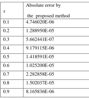
Example 3: Consider the nonlinear boundary value problem
( 9 ) 2 3
, 0 1
y y y c o s x x (30) subject to
( 4 )
( 0 ) 0 , (1) 1, ( 0 ) 1, (1) 1, ( 0 ) 0 , (1) 1,
( 0 ) 1, (1) 1, ( 0 ) 0 .
y y s in y y c o s y y s in
y y c o s y
The exact solution for the above problem is y s in x.
The nonlinear boundary value problem (30) is converted into a sequence of linear boundary value problems generated by quasilinearization technique [3] as
( 9 ) 2 3 2
(n 1 ) (n) (n 1 ) 2 (n) (n) (n 1 ) 2 (n) (n) 0 , 1, 2 , ...
y y y y y y c o s x y y n (31) Subject to
( 1 ) ( 1 ) ( 1 ) ( 1 ) ( 1 ) ( 1 )
( 4 )
( 1 ) ( 1 ) ( 1 )
( 0 ) 0 , (1) 1, ( 0 ) 1, (1) 1, ( 0 ) 0 , (1) 1,
( 0 ) 1, (1) 1, ( 0 ) 0 .
n n n n n n
n n n
y y s in y y c o s y y s in
y y c o s y
0.5 8.696318E-05
0.6 4.911423E-05
0.7 9.953976E-06
0.8 1.654029E-05
0.9 2.005696E-05
x
Absolute error by the proposed method
0.1 4.746020E-06
0.2 1.288950E-05
0.3 5.662441E-07
0.4 9.179115E-06
0.5 1.418591E-05
0.6 1.025200E-05
0.7 2.282858E-05
0.8 1.502037E-05
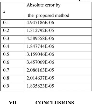
Here y(n1 ) is the (n1)th approximation for y x( ) . The domain [0, 1] is divided into 10 equal subintervals and the proposed method is applied to the sequence of linear problems (31). The obtained numerical results for this problem are presented in Table 3. The maximum absolute error obtained by the proposed method is 2.086163x10⁻⁵.
Table 3: Numerical results for Example 3
VII.
CONCLUSIONS
In this paper, we have developed a collocation method with septic B-splines as basis functions to solve ninth order boundary value problems. Here we have taken mesh points x2,x3, ....,xn2,xn1 as the collocation points. The septic B-spline basis set has been redefined into a new set of basis functions which in number match with the number of selected collocation points. The proposed method is applied to solve several number of linear and non-linear problems to test the efficiency of the method. The numerical results obtained by the proposed method are in good agreement with the exact solutions available in the literature. The objective of this paper is to present a simple method to solve a ninth order boundary value problem and its easiness for implementation.
REFERENCES
[1] Abdel-Halim Hassan, I.H. Vedat Suat Erturk. Solutions of different types of the linear and nonlinear higher order boundary value problems by Differential transformation method, European Journal of Pure and Applied Mathematics, 2009, 2(3), pp.426-447.
[2] Agarwal, R.P. Boundary Value Problems for Higher Order Differential Equations, 1986, World Scientific, Singapore.
[3] Bellal Hossain, M.d. Shafiqul Islam, M.d. A Novel Numerical approach for odd higher order boundary value problems, Mathematical Theory and Modeling, 2014, 4(5) (2014), pp. 1-11.
[4] Bellman, R.E.; Kalaba, R.E. Quasilinearzation and Nonlinear Boundary Value Problems, 1965, American Elsevier, New York.
[5] Chandrashekhar, S. Hydrodynamic and Hydromagnetic Stability, 1981, Dover, New York.
[6] Chawla, M.M., Katti, C.P. Finite difference methods for two-point boundary value problems involving high order differential equations, BIT, 1979, 19, pp. 27-33.
[7] Carl de-Boor. A Pratical Guide to Splines, 1978, Springer-Verlag.
[8] Jafar Saberi-Nadjafi , Shirin Zahmatkesh. Homotopy perturbation method for solving higher order boundary value problems, Applied Mathematical and Computational Sciences, 2010, 1(2), pp.199-224. [9] Luma N.M.Tawfiq, Samaher M.Yassien, Solution of higher order boundary value problems using
Semi-Analytic technique, Ibn Al-Haitham Journal for Pure and Applied Science, 2013, 26(1) , pp. 281-291. [10] Reddy, J.N. An Introduction to the Finite Element Method, 3rd Edition, 2005, Tata Mc-GrawHill
Publishing Company Ltd., New Delhi.
[11] Prenter, P.M. Splines and Variational Methods, 1989, John-Wiley and Sons, New York. [12] Samir Kumar Bhowmik. Tchebychev polynomial approximations for mth order boundary value
problems, International Journal of Pure and Applied Mathematics, 2015, 98(1), pp. 45-63. [13] Schoenberg, I.J. On Spline Functions, MRC Report 625, 1966, University of Wisconsin.
x
Absolute error by
the proposed method
0.1 4.947186E-06
0.2 1.312792E-05
0.3 4.589558E-06
0.4 1.847744E-06
0.5 3.159046E-06
0.6 3.457069E-06
0.7 2.086163E-05
0.8 2.014637E-05
[14] Syed Tauseef Mohyud-Din, Ahmet Yildirim. Solution of tenth and ninth order boundary value problems by homotopy perturbation method, J.KSIAM, 2010, 14(1), pp.17-27.
[15] Syed Tauseef Mohyud-Din, Ahmet Yildirim. Solutions of tenth and ninth order boundary value problems by modified variational iteration method method, Applications and Applied Mathematics: An International Journal (AAM), 2010, 5(1) , pp.11-25.