Convergence Analysis of Moving Object Tracking
Algorithm in 3D using modified EKF based on Bearing
and Elevation Measurements for Underwater
Environment
Nagamani Modalavalasa
1, G. Sasi Bhushana Rao
2and K. Satya Prasad
31
Dept.of ECE, SBTET, Andhra Pradesh, India, , e_mail: [email protected]
2
Dept. of ECE, Andhra University, Visakhapatnam, Andhra Pradesh, India
3Dept.of ECE, Jawaharlal Nehru Technological University Kakinada, Kakinada, India
Abstract-- Underwater surveillance is the primary challenge
being faced by the researchers, scientists and marine community, which include surveillance of harbour, detection of mines, inspecting pipelines and mapping of ocean bottoms etc. The underwater surveillance is best undertaken by the Autonomous Underwater Vehicle (AUV) as it avoids the involvement of human. It is important to note that the convergence time plays very important role in aiding the AUV for its safe navigation as the AUV requires the sufficient time to maneuvering itself for avoiding the objects that comes into its path. Towards this various methods / techniques such as Least Squares (LS), Kalman Filter (KF) and Extended Kalman Filter (EKF) methods have been explored, however all these methods have their own drawbacks. In this paper a new method has been developed wherein tracking algorithm using EKF has been extended to the Bearing and Elevation only Tracking (BEOT) method. The performance of this algorithm has been evaluated using Monte Carlo Method. The convergence issues associated with the new designed algorithm have also been analysed and it has been observed that the errors are considerably small and settles down after the filter learns the existing dynamics.
Index Term— Underwater Vehicle, Tracking, Kalman Filter, BEOT.
I. INTRODUCTION
Tracking underwater objects is an ongoing challenge for safe navigation of AUV. Bearing only tracking (BOT) is used in many marine applications such as sonar based robotic navigation, infrared seeker based tracking and underwater weapon systems. The bearing and elevation only filtering problem in 3D from a single maneuvering sensor is the counterpart of the bearing only filtering in 2D. The important field of research in the areas of aircraft surveillance, submarine tracking, mobile systems and autonomous robotics applications is passive target tracking of maneuvering objects using line of sight (LOS) angle measurements [1-5].
Tracking in underwater environments, where objects have multiple degrees of freedom or when the scene conditions cannot be controlled is much harder. The bearing and elevation only tracking in 3D is much difficult than bearing only tracking in 2D. This is due to the fact that the dynamic model of 3D is not such a straight forward model as in 2D. With this sense the robotic platform could estimate its relative velocity and position with respect to objects within its environment. This would be useful both for navigation and interaction with objects in the environment. Autonomous Underwater Vehicle is a robot, designed to perform specific tasks in underwater. The range, bearing and elevation measurements are often noisy due to turbid nature of underwater environment and results a nonlinear relation between the states and measurements. Due to these measurement inaccuracies gives a direct impact on the performance of the tracking algorithm.
There are two approaches that are generally used in the underwater environment. First approach is the Linear Kalman filter (KF) [6], which was designed by R.E. Kalman in 1960. In this approach measurements are linear and designed for prediction and estimation problem. It can be defined as an optimal recursive data processing algorithm and is characterized by accurate estimation of state variables under noisy condition. It is acceptable for robotic manipulators, drives and other industrial applications. The algorithm is developed in two steps which involve prediction and updating. The second approach is Extended Kalman Filter (EKF) [7] and measurements are nonlinear. It is well organized fact that in EKF the initial covariance is based on the initial converted measurement and the gain is based on the accuracies of the subsequent linearization and therefore the overall performance depends on these accuracies.
Constant Velocity Model (NCVM) and nonlinear measurement model[9]. For 2D tracking problems, Extended Kalman Filter (EKF), Unscented Kalman Filter (UKF), Cubature Kalman Filter (CKF) and Gauss-Hermite Kalman Filter (GHKF) are implemented [10 and 11] .
EKF is implemented for both the predicted state estimate and covariance using a discretized linear approximation[12]. The approaches which are mentioned earlier uses a 2D state estimation problem. The performance of the EKF, UKF and Particle Filter (PF) are compared for the angle-only filtering problem in 3D using bearing and elevation measurements from a single maneuvering sensor[13]. Estimation of the kinematics, such as position and velocity of a target, using noisy-corrupted measurements of the target from a single observer is a nonlinear function.
In the primary research, the EKF algorithm results uncertain performances, including poor track accuracy and divergences [7,8]. A new method has been developed in this research wherein tracking algorithm using EKF has been extended to the Bearing and Elevation only Tracking (BEOT) method. In this approach a single maneuvering sensor/observer case was examined. Also BEOT problem was analyzed with good accuracy and efficiency as the inaccuracies can be tackled effectively in this method.
The target tracking basics is covered in [14]. Most aspects of tracking covered in [15] . Comparison of different tracking methods presents in [16][17] derives a tracking filter that is well suited for angle-only target tracking. The approach that has been followed in this paper is that the non linearities are modified prior subjecting to the tracking algorithm with angles only measurements. Modified gains for the bearings and elevation problem have also been derived in a simplistic manner. The results have been promising and have shown improved performance over the conventional EKF.
Song T.L. and Speyer LL derived a modified gain extended kalman filter (MGEKF) for nonlinear estimation problems[18]. This MGEKF algorithm was further developed by Galkowiski P.J. and Islam M.A. based on the pseudo measurements[19]. Mo, Longbin, Liu, Qi, Zhou, Yiyu, Sun, Zhongkang presented the improved modified gain functions for 3D angles-only tracking[20][21]. In this paper the nonlinearities are modified and then applied to a tracker with bearing and elevation only measurements. It shows an improved performance over the conventional Extended Kalman Filter (EKF). In this paper, modified gains for the bearings and elevations problem have been derived in a simpler manner .
II. TRACKING ALGORITHM
The primary problem in bearing and elevation only tracking is to estimate the trajectory of the object/target from noisy corrupted sensor data[22]. In this scenario the observer tracks a moving target/object with sensor(sonar), which measures only the bearings and elevations of the target with respect to positions of the sensor. There is one moving target/object in the scene and one sensor(sonar) for tracking it. The state of the Target Motion Model (TMM) is described by a Nearly Constant Velocity Model (NCVM) and at time step (k+1) consists of the position in three dimensional (3D) Cartesian
coordinates , and and the velocity towards those coordinate axes , and . Thus, the dynamics of the target is modeled as a state space model. The state of the target is defined in the tracker coordinate frame (T frame) for which the x, y , and z axes are along the local North, East and upward directions, respectively as shown in Fig.1. The target and sensor/observer states in Cartesian coordinates are defined as follows
(1)
And
(2)
The relative state vector in the T frame is defined by
(3)
Let the relative state vector in the T frame is
(4)
Then, , , etc.
The range vector of the target from the observer ( or sensor) in the T frame is,
= = (5)
Then the range is defined as
= √ (6)
The range vector can be expressed in terms of range, bearing ( ) and elevation ( ), as defined in Figure 1, by
= [
] (7)
Target Motion Model (TMM) is described in the Cartesian coordinate system by linear discrete–time difference equation with some additive noise as
( ) ( ) ( ) ( ) (8)
Where, the state vector ( ) consists of the position and velocity components of the target moving in the 3-D space.
i.e. ( ) ( ) ( ) ( ) ( ) ( ) ( ) (9)
( ) ( ) (10) ( ) [ ] (11)
The target is tracked by a Sonar in the underwater and provides measurements of bearing ( m) and elevation ( m).
The measurement model is given as
( ) ( ) ( ) (12)
( ) [ ( )( )] [ ( ) ( ) √ ( ) ( ) ( ) ] (13) Where ( )is uncorrelated, zero-mean white Gaussian noise with variances , in the bearing ( ) and elevation ( ) measurements respectively .
The measured range, bearing, and elevation from sonar are converted to target positions in Cartesian coordinates with respect to own ship as origin using the following relations:
( )
( )
( )
( ) ( ) ( ) (14)
Where, is the range vector of x, y and z positions.
Because the measurement model is non-linear we replace the Kalman filter algorithm with EKF. The dynamic model using NCVM in 3D is linear and the measurement model for bearing and elevation is nonlinear for this problem. In general EKF is based on linearized approximations to nonlinear dynamic and/or measurement models [9], [23] and is widely used. For this problem, the linearized approximation is performed in the measurement update step as described in [9], [23].
With the designed system dynamic and measurement model given in Eq.(8) and Eq.(12), the process of estimating state vector
x
(k)with the proposed BEOT algorithm is elucidated in Eq.(15) to Eq.(19). The algorithm estimates state vector 1) (k
x
, from the initial state estimatex
(k)and its uncertainty matrixP
(k) as given in Eq.(15) and Eq.(16). Kalman gain in Eq.(17) is the function of uncertainty in state estimate and measurement error , provides weight coefficients to the measurements at time (k+1) used for state vector updationgiven in Eq. (17). The updated state covariance matrix at time (k+1) is a function of modified gain
g
and is shown in Eq.(19). ) ( ) 1 ( ) 1(k
F
kx
kx
(15)) 1 ( ) 1 ( ) ( ) 1 ( ) 1 (
kT k k k
k
F
P
F
Q
P
(16))
(
( 1) ( 1) ( 1)) 1 ( ) 1 ( ) 1 (
k
k k
k kk
x
K
z
H
x
x
(17))
(
( 1) ( 1) ( 1)) 1 ( ) 1 ( ) 1 (
R
H
P
H
H
P
K
T k k k T k kk
(18)
T k k T k k k k k k k k
K
R
K
x
z
g
K
I
P
x
z
g
K
I
P
) 1 ( ) 1 ( ) 1 ( ) 1 ( ) 1 ( ) 1 ( ) 1 ( ) 1 ( ) 1 ( ) 1 ()
,
(
(
)
,
(
(
(19) Where , ) (kx
= State estimate at time k.) 1 (k
F
= State transition matrix at time k+1. 1) (k
x
= Predicted state estimate at time k+1.) (k
P
= State covariance matrix estimate at time k. 1) (k
P
= Predicted state covariance matrix at k+1 time.) 1 (k
Q
= Process noise covariance matrix at k+1time.) 1 (k
x
= Updated state estimate at time k+1 .) 1 (k
K
= Filter gain at time k+1.) 1 (k
z
= Measurement data at time k+1.) 1 (k
H
= Measurement matrix at time k+1.) 1 (k
P
=Updated state covariance matrix at time k+1.R
= Measurement noise covariance matrix.)
,
(
z
(k1)x
(k1)g
= Modified gain function.I
= Identity matrix.The main difference between the EKF and MGEKF is the function
g
in the covariance update.To determine the modified gain function
g
we write:[( ̂)( ̂)]
g
[ ( ̂) ( ̂) ( ̂)](20)
Since ‘
g
’ is not a function of target velocity we removed those states for the derivation of ‘g
’.The measurement matrix H is given by
[
̂ ̂
̂ ̂
̂̂ ̂
̂ ̂ ̂
̂ ̂
] (21)
III. UPDATED MEASUREMENT OF BEARING DATA
If the range in horizontal plane is
= √
Then the estimated range be
̂ = √ ̂ ̂
By adding with ̂ we can get,
+ ̂ = + + ̂ ̂ + ̂ ̂ (22)
Adding both sides with ̂ - ̂ - ̂ - ̂
+ ̂ =( ̂)( ( ̂ ) ( ̂)( ̂) ̂) (23)
Similarly,
- ̂ =( ̂) ( ( ̂) ( ̂)( ̂) ̂) (24)
2 ̂ =( ̂) [ ̂
( ̂ )
̂
( ̂)]+
( ̂) [ ( ̂)̂ ( ̂)̂] (25)
Taking Eq. (25) and simplifying we get
[ ( ̂)̂ ( ̂)̂] = -2 ( ( ̂) ̂) ̂
= -2
( ̂) (26)
[ ( ̂)̂ ( ̂)̂] = 2 ( ( ̂ ) ̂ ) ̂
= 2
( ̂ ) (27)
Now the coefficients of
( ̂)
and( ̂)
are then,̂ = ( ̂)( ̂) +
( ̂)( ̂) (28)
Equation (28) rewritten as
( ̂) = ( ̂) ( ̂)
̂ (29)
IV. UPDATED MEASUREMENT OF ELEVATION DATA
As can be seen from the above analysis
= generates
( ̂) = ( ̂) ( ̂)
̂ (30)
In the similar way
√ =
= generates,
( ̂) = ( ̂) ̂ ( ̂ )
(31)
From the Eq. (24) we get
- ̂ =
( ̂) ( ̂) ( ̂) ( ̂)
( ̂) (32)
Now replacing Eq. (32) in Eq. (31),
( ̂)= ( ̂)
̂
̂ [
( ̂) ( ̂) ( ̂) ( ̂)
( ̂) ]
(33)
By rearranging the Eq. (33) becomes,
( - ̂) (
̂
)
̂ ( - ̂)
( - ̂) ( ̂
)
̂ ( ̂) ( ̂)
( ̂) ̂
(34)
[( ̂) ( ̂)]
[
̂
̂
( ̂)
̂ ( ̂)
( ̂)
̂ ( ̂)
̂ ]
[ ( ̂) ( ̂) ( ̂)
]
(35)
compute the modified gain. Hence the Eq. (35) can be rewritten as,
[( ̂)( ̂)]
[
̂
̂
( ̂)
̂ ( ̂)
( ̂)
̂ ( ̂)
̂ ]
[ ( ̂) ( ̂) ( ̂)]
(36)
By considering the velocity components
g
is given by
g
=[
̂
̂
(
̂)
̂ ( ̂)
( ̂)
̂ ( ̂)
̂
]
(37)
V. RESULTS AND DISCUSSIONS
When extending the 2D estimation to 3D estimation, it is important to redefine the parameters of target and observer. For the validation of the proposed algorithm the simulation has been generated with different measurement inaccuracies with simulated data. Own-ship is always considered at the origin and also assumed that the target is moved with constant velocity and travels in a straight path. The tracking angles of the observer and target are shown in Fig.1.
Initial SONAR signal assumptions considered for the simulations are,
1. Always own ship is at origin(O i.e. sonar at (0,0,0) coordinates).
2. Target is moving at constant speed.
3. All angles (Bearing and Elevation angles) are considered with respect to target.
For the implementation of the algorithm, the initial estimate of target state vector is chosen as follows. As only bearing and elevation measurements are available, it is not possible to guess the velocity components of the target. So these components are assumed as 10 m/s; which are close to the realistic speeds of the vehicles in underwater environments.
Fig. 1 Tracking Angles
The initial state has been defined as,
(38)
Where and are initial bearing and elevation measurements.
Initial target velocity = 10 m/sec. Initial target course = 135 deg. Initial target range = 10km. Initial target bearing = 0.5 deg. Initial target elevation = 45 deg.
= 0.0015 = 30 = 0.0015
Where, and are the variances in range (r), bearing ( ) and elevation ( ) respectively.
The noise in the bearing is assumed to be additive in nature and follows normal distribution. The measurement contains noise generated by several noise sources according to central limit theorem, i.e. the sum of noises of any density function leads to Gaussian density function. So, it is assumed that the noises in the measurements are of Gaussian nature. Many random processes occurring in nature actually appear to be normally distributed. So the noise in the bearing is assumed to be additive in nature and follows normal distribution.
Bearing and elevation measurements are taken for every 1 second for 1000 Monte Carlo updates. Fig. 2 shows the trajectories of ownship, true target and predicted target. Initial covariance matrix is assumed as per the standard procedure in [24].
XY plane
P( 𝑥 𝑦)
𝜃 𝜑
𝑦
P( 𝑥 𝑦,z) 𝑋
𝑧 𝜃 P( 𝑥 z)
𝑂 𝑥
𝑟 𝑥𝑦𝑧
𝑟 𝑥𝑦 𝑍
Fig. 2. Observer, True Target and Predicted Target Trajectories
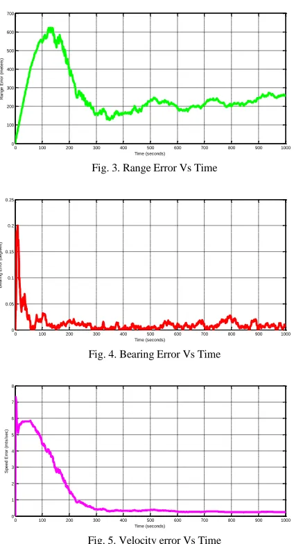
Fig. 3. Range Error Vs Time
Fig. 4. Bearing Error Vs Time
Fig. 5. Velocity error Vs Time
Fig. 6. Course Error Vs Time
The estimated errors in simulations 1 are plotted in Fig.3 to Fig.7. It has been observed that the convergence duration is 300 seconds in case of range, 80 seconds in case of bearing, 200 seconds in case of velocity, 800 seconds in case of course and 800 seconds in case of elevation, which indicate the suitability of this method for aiding the AUV for its safe navigation.
Fig. 7. Elevation Error Vs Time
The performance of the algorithm is evaluated in terms of : i. The percentage fit error (PFE) in and
( ̂) ( ) (38)
( ̂) ( ) (39)
( ̂) ( ) (40)
ii. The root mean square position error
√ ∑ ( ̂) ( ̂) ( ̂ ) (41)
Where, N= 1,2,3…1000 Monte Carlo runs.
iii. The root mean square velocity error
√ ∑ ( ̂ ) ( ̂ ) ( ̂ ) (42)
Where, N= 1,2,3…1000 Monte Carlo runs.
iv. The root sum square position error
0 50
100 150
200
0 2000 4000 6000 8000
0 0.5 1 1.5 2
x 104
ry (metres) rx (metres)
rz
(
m
e
tr
e
s
)
Simulated Target Trajectory Predicted Target Trajectory Observer Position
0 100 200 300 400 500 600 700 800 900 1000
0 100 200 300 400 500 600 700
Time (seconds)
R
a
n
g
e
E
rr
o
r
(m
e
te
rs
)
0 100 200 300 400 500 600 700 800 900 1000
0 0.05 0.1 0.15 0.2 0.25
Time (seconds)
B
e
a
ri
n
g
E
rr
o
r
(d
e
g
re
e
s
)
0 100 200 300 400 500 600 700 800 900 1000
0 1 2 3 4 5 6 7 8
Time (seconds)
S
p
e
e
d
E
rr
o
r
(m
ts
/s
e
c
)
0 100 200 300 400 500 600 700 800 900 1000
0 20 40 60 80 100 120 140
Time(seconds)
C
o
u
rs
e
E
rr
o
r
(d
e
g
re
e
s
)
0 100 200 300 400 500 600 700 800 900 1000
0 5 10 15 20 25 30 35 40 45
Time(seconds)
E
le
v
a
ti
o
n
E
rr
o
r
(d
e
g
re
e
s
√( ̂) ( ̂) ( ̂) (43)
v. The root sum square velocity error
√( ̂ ) ( ̂ ) ( ̂) (44)
where and are the measurements, ̂ ̂ and ̂ are the estimated target positions, and are the measurements, ̂ ̂ and ̂ are the estimated target velocities in and
coordinates, respectively. Here RMSPE, RMSVE, RSSPE and RSSVE are calculated at each time step as given in the equations (41 & 44).
The Percentage Fit errors and Mean absolute errors in x, y and z positions of scenario1 are plotted in Fig. 8 and Fig. 9 and found to be in acceptable ranges. The Root Mean Square Errors in position (RMSPE) and velocity (RMSVE), Root Sum Square Errors in position (RSSPE) and velocity (RSSVE) are shown in Fig.10. It is observed that the errors are small and settled down after filter learns dynamics.
Root sum square position errors in x, y and z positions are shown in Fig.11 and observed that the errors are small.
Fig. 8. Percentage fit errors in x, y and z positions
Fig. 9. Mean absolute errors in x, y and z positions
Fig. 10. RMSP, RMSV, RSSP and RSSV in predicted position
Fig. 11. RSSP in x, y and z positions for simulation 1
Comparison of Proposed BEOT algorithm with Conventional EKF:
The computational time of Extended Kalman Filter (EKF) is generally less when compared to Unscented Kalman Filter(UKF) and Particle Filter ( PF) [25, 26]. In real time scenario the computational time is more important than the accuracy of the position estimation. Because of this reason the results of the proposed algorithm are not compared with the UKF and PF.
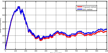
In Fig. 12 to Fig. 16 the range, bearing, velocity, course and elevation errors for proposed BEOT method is compared with conventional EKF method for every time step of 1000 Monte Carlo runs and found to be optimum.
It is observed that the range, bearing, velocity, course and elevation errors are optimum for the proposed algorithm.
Fig. 12. Range error of proposed BEOT algorithm and EKF
0 100 200 300 400 500 600 700 800 900 1000
0 0.2 0.4
P
F
E
x
0 100 200 300 400 500 600 700 800 900 1000
0 5 10
P
F
E
y
0 100 200 300 400 500 600 700 800 900 1000
0 0.2 0.4
P
F
E
z
time in sec.
0 100 200 300 400 500 600 700 800 900 1000
0 0.5 1
M
A
E
x
0 100 200 300 400 500 600 700 800 900 1000
0 0.5 1 1.5
M
A
E
y
0 100 200 300 400 500 600 700 800 900 1000
0 0.5 1
M
A
E
z
time in sec.
0 100 200 300 400 500 600 700 800 900 1000
0 20 40
R
S
S
P
E
0 100 200 300 400 500 600 700 800 900 1000
0 5 10
R
M
S
P
E
0 100 200 300 400 500 600 700 800 900 1000
0 0.5 1
R
M
S
V
E
0 100 200 300 400 500 600 700 800 900 1000
0 1 2
R
S
S
V
E
time in sec.
0 100 200 300 400 500 600 700 800 900 1000
0 10 20 30
R
S
S
P
E
x
0 100 200 300 400 500 600 700 800 900 1000
0 5 10
R
S
S
P
E
y
0 100 200 300 400 500 600 700 800 900 1000
0 10 20 30
R
S
S
P
E
z
time in sec.
0 100 200 300 400 500 600 700 800 900 1000 0
100 200 300 400 500 600 700
Time (seconds)
R
a
n
g
e
E
rr
o
r(
m
e
te
rs
)
Fig. 13. Bearing error of proposed BEOT algorithm and EKF
Fig. 14. Velocity error of proposed BEOT algorithm and EKF
Fig. 15. Course error of proposed BEOT algorithm and EKF
Fig. 16. Elevation error of proposed BEOT algorithm and EKF
The same algorithm is validated practically with the sector scan sonar that operates with the ranges of 100m and 300m. The sonar which was used to collect the data is Super Seeking DST (Digital Sonar Technology) Dual Frequency CHIRP Sonar. Sector scan sonar with the following specifications: Operating frequency (low)-Chirping from 250 to 350 kHz (300kHz).
Operating frequency (high)-Chirping from 620 to720 kHz (670kHz).
Optional high frequency is 1 MHz. Maximum range is 300 m [300kHz]. Maximum range is 100 m [670kHz].
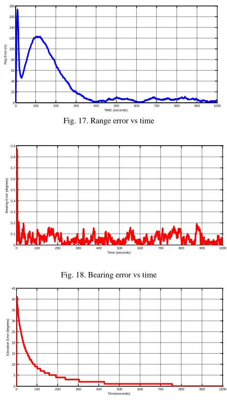
The simulated results with the assumed data and the results obtained from the Sector Scan Sonar(SSS) data are similar. The following figures corresponding to SSS data. Fig. 17 to Fig.19 shows the range, bearing and elevation errors.
Fig. 17. Range error vs time
Fig. 18. Bearing error vs time
Fig. 19. Elevation error vs time
VI. CONCLUSIONS
In this paper , simulations has been done in 3D estimation algorithms based on the 2D estimation BOT problem. A new Bearing and Elevation only Tracking algorithm was designed using modified kalman gain to evaluate the system performance and has been developed for underwater object detection/tracking. The experimental results also show with 1000 Monte Carlo simulations and the convergence issues associated with the developed algorithm has been analyzed. It
0 100 200 300 400 500 600 700 800 900 1000 0
0.05 0.1 0.15 0.2 0.25
Time (seconds)
B
e
a
ri
n
g
E
rr
o
r(
d
e
g
)
Proposed method EKF method
0 100 200 300 400 500 600 700 800 900 1000 0
1 2 3 4 5 6 7 8
Time (seconds)
S
p
e
e
d
E
rr
o
r(
m
/s
e
c
)
Proposed method EKF method
0 100 200 300 400 500 600 700 800 900 1000 0
20 40 60 80 100 120 140
Time (seconds)
C
o
u
rs
e
E
rr
o
r(
d
e
g
)
Proposed method EKF method
0 100 200 300 400 500 600 700 800 900 1000
0 5 10 15 20 25 30 35 40 45
Time (seconds)
E
le
v
a
ti
o
n
E
rr
o
r(
d
e
g
)
Proposed method EKF method
0 100 200 300 400 500 600 700 800 900 1000
0 20 40 60 80 100 120 140 160 180
TIME (seconds)
R
n
g
E
rr
o
r
(m
)
0 100 200 300 400 500 600 700 800 900 1000 0
0.1 0.2 0.3 0.4 0.5 0.6 0.7 0.8 0.9
Time (seconds)
B
e
a
ri
n
g
E
rr
o
r
(d
e
g
re
e
s
)
0 100 200 300 400 500 600 700 800 900 1000
0 5 10 15 20 25 30 35 40 45
Time(seconds)
E
le
v
a
ti
o
n
E
rr
o
r
(d
e
g
re
e
s
is found that the errors are small and settle down after the filter learns the dynamics and will converge more quickly.
In real time underwater scenario the computational time is more important than the accuracy of the state error rate. The results of the proposed BEOT method are compared with the traditional EKF algorithm and observed that range, bearing, velocity, course and elevation errors of the target are optimum.
The same algorithm is validated practically with the sector scan sonar that operates with the ranges of 100m and 300m. It is also observed that the simulated results with the assumed data and the results obtained from the Sector Scan Sonar(SSS) data are similar.
Acknowledgements
This research paper has resulted from the NSTL (DRDO), Visakhapatnam, Andhra Pradesh, INDIA sponsored research project.
REFERENCES
[1] Goutam Chalasani,, Shovan Bhaumik, “Bearing Only Tracking Using Gauss-Hermite Filter” IEEE, 2011 ISSBN:978-1-4577- 2119
[2] S.Sadhu, S.Bhaum` ik, and T.K.Ghoshal, “Evolving homing guidance configuration with Cramer Rao bound,” Proceedings 4th IEEE International Symposium on Signal
Processing and Information Technology, Rome, 18th-21st
December 2004.
[3] T.L.Song, and J.L.Speyer, “A stochastic analysis of a modified gain extended Kalman filter with applications to estimation with bearing only measurements”, IEEE Trans. Autom. Contmi, 1985, AC-30, No.10, October 1985, pp. 940-949.
[4] Ronghui Zhan and Jianwei Wan, “Passive maneuvering target tracking using 3D constant- turn model”, Radar, 2006, IEEE Conference.
[5] K. Dogancay, 2005 “Bearings-only target localization using total least squares,” Signal Process, vol. 85, pp.
1695-1710.
[6] R. E. Kalman, “A new approach to linear filtering and prediction problems,” ASME J. Basic Eng.,1960.
[7] Nardone, S. C., Lindgren, A. G., and Gong, K.F., Fundamental properties and performance of conventional bearings-only target motion analysis. IEEE Transactions on Automatic Control, AC-29,Sept. 1984 9, pp. 775—787.
[8] V. J. Aidala, “Kalman filter behavior in bearing-only tracking applications”, IEEE Trans. on Aerospace and Electronic Systems, Vol. AES-15, No. 1, January 1979, pp. 29–39.
[9] Y. Bar-Shalom, X. R. Li, and T. Kirubarajan, “Estimation with Applications to Tracking and Navigation”, John Wiley & Sons, 2001.
[10] B. L. Scala, M. Morelande, “An Analysis of the Single Sensor Bearings-Only Tracking Problem”, Information fusion, 11th
international conference, 2008 .
[11] Jouni Hartikainen, Arno Solin, and Simo Sarakka, “Optimal filtering with Kalman filters and smoothers, A manual for the Matlab tool box”, Aalto-Finland, August 2011.
[12] R. Karlsson and F. Gustafsson, ”Range estimation using
angle-only target tracking with particle filters”, Proc. American Control Conference, 2001, pp. 3743 – 3748.
[13] Mallick, M., Morelande, M.R., Mihaylova and L, Arulampalam,
S., Yan, “Comparison of Angle-only Filtering Algorithms in 3D
using Cartesian and Modified Spherical Coordinates”, 15th
International Conference on IEEE, 2012, pp. 1392-1399.
[14] Y. Bar-Shalom and X. Li. “Estimation and Tracking Principles, Techniques,and Software,” Artech House, 1993.
[15] S. Blackman and R. Popoli. “Design and Analysis of Modern Tracking Systems,” Artech House, 1999.
[16] B. Ristic, S. Arulampalam, and N. Gordon, “Beyond the Kalman Filter, Particle Filters for Tracking Application,” Artech House, 2004.
[17] V. J. Aidala and S. E. Hammel “Utilization of Modified Polar Coordinates for Bearings-Only Tracking,” In IEEE Transaction on Automatic Control, volume AC-28, March 1983.
[18] T.L.Song, and J.L.Speyer “A stochastic analysis of a modified gain extended Kalman filter with applications to estimation with bearing only measurements,” IEEE Trans. Autom. Contmi, 1985, AC-30, No.10, October 1985, pp 940-949.
[19] PI. Galkowski, and M.A. Islam, “An alternative derivation of the modified gain function of Song and Speyer,” IEEE Trans. Autom Control, 1991, Vol.36, Issue 11, pp. 1323-1326.
[20] Mo, Longbin, Liu Qi, Zhou Yiyu, Sun, Zhongkang, “New modified measurement function in 3D passive tracking”, Acquisition, Tracking and Pointing XI, Proc. SPIE, Vol. 3086, pp. 311-314.
[21] MO Longbin, Liu Qi, Zhou Yiyu and Sun Zhongkang, “Utilization of the Universal Liniarization in target tracking”, IEEE Transactions on Aerospace and Electronics conference, 1997.
[22] K. Radhakrishnan, A. Unnikrishnan, and K.G Balakrishnan, “Bearing only Tracking of Maneuvering Targets using a Single Coordinated Turn Model”, International Journal of Computer Applications, 2010.
[23] A. Gelb, editor, Applied Optimal Estimation, MIT Press, 1974. [24] Y. T. Chan and S.W. Rudnicki, “Bearings -only Doppler Bearing
Tracking using Instrumental Variables”, IEEE Transactions on Aerospace and Electronic Systems, Vol.28, No.4, October 1992. [25] T. Fiorenzani. C.Manes, G. Oriolo and P.Peliti, “Comparative
study of Unscented Kalman Filter and Extended Kalman Filter position/attitude estimation in unmanned aerial vehicle”, Itallian National research Council ( IASI-CNR,), ISSN: 1128-3378.