Abstract— In this research, the manufacturing complexity of the Saudi Airlines Engineering Industries (SAEI) is measured to determine the complexity of their maintenance plants. We analyze the results based on the measurement of the complexity model to determine the most influential operations affecting the maintenance process and causing delays using the Pareto analysis (ABC analysis). When the complexity is considered for the planned and actual durations, there is no part mix ratio available for the data, and the planned and actual durations result in minor complexity measurements. The levels of complexity for the planned and actual durations are 1.375 and 2.1123, respectively. An ABC analysis is also conducted, and the results indicate that certain processes affect both plans.
Index Term— Complexity; Pareto Analysis; ABC analysis;
I. INTRODUCTION
TODAY’S dynamic environment makes it difficult for factories and manufacturing plants to achieve their objectives. To achieve these targets, factories and manufacturing plants are often required to perform at their best capabilities. To survive with the changing environment, companies objectives to be more flexible in their processes and systems to fulfill customers’ demands. This flexibility may yield benefits, such as increased production and product customization. However, if not controlledorganized, such flexibility might lead to higher costs, longer lead times, , larger inventories, and customer dissatisfaction.
This study has two aims. The first objective is to measure the complexity of maintenance lines. Saudi Airlines Engineering Industries (SAEI) has provided us with the data for one maintenance line. The line has a different number of processes. The second objective is to determine the factors that can help reduce the complexity of these lines. Such a reduction can be realized in many ways, such as JIT, product & process standardization and other techniques used for complexity management. However, these methods do not answer the following question: How complex is the system and to what degree can the complexity be reduced? Changing the part mix ratio can help to reduce the complexity level.
The main objectives of the study are to
1. Measure the complexity of maintenance lines.
R. Alamoudi is with the Department of Industrial Engineering, King Abdulaziz University, Jeddah, Saudi Arabia.
M. Balubaid are with the Department of Industrial Engineering, King Abdulaziz University, Jeddah, Saudi Arabia (e-mail: [email protected]).
2. Determine the factors that can help reduce the complexity of these lines.
II. LITERATURE REVIEW
In this section, we discuss the various definitions of complexity and attempt to identify the characteristics of complexity and complex systems. We provide a brief overview of the literature on complexity to lead into the proposed model of measuring the complexity of manufacturing systems.
According to Park and Kermer [1] there is no widely accepted common definition of complexity due to the vagueness that the term itself has.. Weaver [2] explained that a complex system is a large number of parts that interact in a non-simple manner. Yates [3] states five characteristics of complex systems. He proposed that complexity rises whenever one or more of the following five characteristics are present: (a) significant interactions; (b) high number of parts, degrees of freedom, or interactions; (c) non-linearity; (d) broken symmetry; and (e) non-holonomic constraints. Allen and Torrens [4] define a complex system as one that can respond in more than one way to its setting.
Acorrding to Sedra [5], the main characteristics of complex systems are collected under structural (static) and behavioral (dynamic) features in the literature. The structural feature of complexity illistrate the number of parts, variety of parts, strength of interactions, connective structure, and hierarchical structure (see Table I). The behavioral aspect involves the characteristics of dynamism, nonlinearity, being far from equilibrium, historicity, adaptively, self-organization, emergent structures, and evolution (see Table II).
TABLEI
STATIC CHARACTERISTICS OF EVALUATING COMPLEX SYSTEMS
Measuring the Complexity in an Airplane
Engine Maintenance Plant
TABLEII
DYNAMIC CHARACTERISTICS OF EVALUATING COMPLEX SYSTEMS
Park and kremer [1] discussed that complexity for manufacturing systems can be categorized into two broad main areas equivalent to application or focus areas: design complexity and manufacturing complexity. In addition Park and Kremer [1] discussed how these types of complexity have been defined beyond ambiguous and quantified through different approaches.
Research have showed that complexity can affect a manufacturing company’s performances, and those of its supply chain [6]. Where Perona and Miagliotta [6] model suggests that the ability to control complexity within manufacturing and logistic systems can improve efficiency and effectiveness at a supply chain wide scale.
Deshmukh et al. [7] have formulated an entropic measure for static manufacturing complexity. However, it is designed to be applied to only flexible manufacturing systems (FMSs).
Cho et al [8] proposed a novel model that can capture both direct and indirect interactions among resources, which are not limited to machining or forming operations.
We will apply this model in the current study. An explanation of the model is provided in the next part.
A. Measurement Using a Complexity
1. Let us consider a manufacturing system that produces n different types of parts and consists of m machines. 2. The interaction index matrix, which accounts for the existence of interactions among processes in terms of the processing time and waiting time (l), will be:
(1)
3. Matrix (Pl) is called the processing time matrix, where diagonal elements represent processing times and off-diagonal elements are zeros and is given as
(2) 4. The interaction matrix ( l), which represents
processing based interaction and waiting time-based interaction, is given as
(3)
5. The total interaction matrix is
(4) When we consider part mix ratios if they exist in the model, then the overall interaction matrix will be
(5)
where
6. The normalized direct interaction matrix is
(6)
where
7. The normalized general interaction matrix is
(7) which reflects all higher-order (indirect) interactions over k connections (arcs), i.e., k=1 corresponds to direct interactions, k=2 corresponds to second-order interactions over 2 connections, and so on.
8. The overall influence of the i-th machine in the
system is (8)
l
jlijlil=0 1
ì í î
n n
i l l
n
l l
P Λ P
Λ P Λ Π
Π
1 1 1 1
y
l=
1
l=1n
å
ˆ
π
i
=
p
ˆ
ij
j
=
1
m
å
Indices to show
self-interaction in terms
of process time.
Indices for influence of
machine
of machine
in terms of waiting time.
l
jli+1jlil=
9. The normalized influence of the i-th machine in the
system is (9)
10. Finally, the static complexity can be calculated using Shannon’s entropy theorem:
(10) III. COMPLEXITY MODEL
In this section, we measure the manufacturing complexity of the SAEI Airplane Engine Repair Facility using the model presented above. We gathered the data from SAEI. The data are shown below, where the expected starting and ending dates of each process for each module are listed. We were provided with three schedules of three different engines that were processed in one production line.
A. First Engine
The schedule of the first engine detailed with planned and actual dates is shown in Table III.
TABLEIII
FIRST ENGINE PLAN AND ACTUAL DATES OF OPERATION
ST EP S
OPERA TION
PLANNED ACTUAL DURA
TION DIFFE RENCE ST AR T EN D DURA TION ST AR T EN D DURA TION 1
MOD. REMOV AL 1-AP R -14 3-AP R -14 3 1-AP R -14 20-AP R -14
20 -17
2
MOD. DISASS EMBLY 4-AP R -14 8-AP R -14 5 21-AP R -14 28-M AY -14
38 -33
3 CLEANI
NG 9-AP R -14 10-AP R -14 2 29-MA Y -14 30-M AY -14
2 0
4 N.D.T 11-AP R -14 11-AP R -14 1 31-MA Y -14 1-JU N -14
1 0
5 BENCH INSP.
12-AP R -14 14-AP R -14 3 2-JU N -14 4-JU N -14
3 0
6 PARTS REPAIR (MRP) 15-AP R -14 19-M AY -14 35 6-JU N -14 10-JU N -14
5 30
7
QEC PARTS
REP. (R.SHO P) 15-AP R -14 19-M AY -14 35 6-JU N -14 10-JU N -14
5 30
8 PARTS PURCHA SING (SC.) 15-AP R -14 19-M AY -14 35 6-JU N -14 10-JU N -14
5 30
9 PARTS REPAIR (R.SHO P) 15-AP R -14 19-M AY -14 35 6-JU N -14 10-JU N -14
5 30
10 KIT
20-MA Y -14 20-M AY -14 1 11-JU N -14 12-JU N -14
2 -1
11
MOD. ASSEMB LY 21-MA Y -14 30-M AY -14 10 13-JU N -14 23-JU N -14
11 -1
12
MOD. INSTAL LATION 31-MA Y -14 4-JU N -14 5 24-JU N -14 2-JU L -14
9 -4
13 TEST
5-JU N -14 9-JU N -14 5 3-JUL -14 4-SE P -14
64 -59
B. Second Engine
The schedule of the second engine detailed with planned and actual dates is shown in Table IV.
TABLEIV
SECOND ENGINE PLAN AND ACTUAL DATES OF OPERATION
ST EPS
OPERAT ION
PLANNED ACTUAL DURAT
ION DIFFER ENCE STA RT EN D DURA TION STA RT EN D DURA TION 1
MOD. REMOV AL 24-FEB -14 26-FE B -14 3 24-FEB -14 17-M AR -14
22 -19
2
MOD. DISASSE MBLY 27-FEB -14 3-M AR -14 5 18-MA R -14 15-AP R -14
29 -24
3 CLEANI
NG 4-MA R -14 5-M AR -14 2 16-AP R -14 17-AP R -14
2 0
4 N.D.T 6-MA R -14 6-M AR -14 1 18-AP R -14 19-AP R -14
2 -1
5 BENCH INSP.
7-MA R -14 9-M AR -14 3 20-AP R -14 2-M AY -14
13 -10
6 PARTS REPAIR (MRP) 10-MA R -14 13-AP R -14 35 3-MA Y -14 14-JU N -14
43 -8
7
QEC PARTS
REP. (R.SHOP ) 10-MA R -14 13-AP R -14 35 3-MA Y -14 14-JU N -14
43 -8
8 PARTS PURCHA SING (SC.) 10-MA R -14 13-AP R -14 35 3-MA Y -14 14-JU N -14
43 -8
9 PARTS REPAIR (R.SHOP ) 10-MA R -14 13-AP R -14 35 3-MA Y -14 14-JU N -14
43 -8
10 KIT 14- 14- 1 15- 16- 1 0
⌣
p
i
=
p
ˆ
i
ˆ
p
i
i=1
AP R -14 AP R -14 JUN -14 JU N -14 11
MOD. ASSEMB LY 15-AP R -14 24-AP R -14 10 15-JUN -14 1-JU L -14
17 -7
12
MOD. INSTALL ATION 25-AP R -14 29-AP R -14 5 2-JUL -14 9-JU L -14
8 -3
13 TEST
30-AP R -14 4-M AY -14 5 10-JUL -14 14-JU L -14
5 0
C. Third Engine
The schedule of the third engine detailed with planned and actual dates is shown in Table V.
TABLEV
THIRD ENGINE PLAN AND ACTUAL DATES OF OPERATION
ST EPS
OPERAT ION
PLANNED ACTUAL DURAT
ION DIFFER ENCE STA RT EN D DURA TION STA RT EN D DURA TION 1
MOD. REMOV AL 20-JAN -14 22-JA N -14 3 20-JAN -14 27-JA N -14
8 -5
2
MOD. DISASSE MBLY 23-JAN -14 27-JA N -14 5 28-JAN -14 23-FE B -14
27 -22
3 CLEANI
NG 28-JAN -14 29-JA N -14 2 24-FEB -14 25-FE B -14
2 0
4 N.D.T 30-JAN -14 30-JA N -14 1 26-FEB -14 13-M AR -14
16 -15
5 BENCH INSP.
31-JAN -14 2-FE B -14 3 14-MA R -14 19-M AR -14
6 -3
6 PARTS REPAIR (MRP) 3-FEB -14 9-M AR -14 35 20-MA R -14 23-AP R -14
35 0
7
QEC PARTS
REP. (R.SHOP ) 3-FEB -14 9-M AR -14 35 20-MA R -14 23-AP R -14
35 0
8 PARTS PURCHA SING (SC.) 3-FEB -14 9-M AR -14 35 20-MA R -14 23-AP R -14
35 0
9 PARTS REPAIR (R.SHOP ) 3-FEB -14 9-M AR -14 35 20-MA R -14 23-AP R -14
35 0
10 KIT
10-MA 10-M 1 24-AP
10-M 17 -16
R -14 AR -14 R -14 AY -14 11
MOD. ASSEMB LY 11-MA R -14 20-M AR -14 10 11-MA Y -14 19-M AY -14
9 1
12
MOD. INSTALL ATION 21-MA R -14 25-M AR -14 5 20-MA Y -14 24-M AY -14
5 0
13 TEST
26-MA R -14 30-M AR -14 5 25-MA Y -14 28-JU N -14
33 -28
D. List of Processes
The list of processes is shown in Table VI. TABLEVI
LIST OF PROCESSES
# PROCESSES
1 MOD.REMOVAL
2 MOD.DISASSEMBLY
3 CLEANING
4 N.D.T
5 BENCH INSP.
6
PARTS REPAIR (MRP) QECPARTS REP. PARTS PURCHASING
PARTS REPAIR
7 KIT
8 MOD.ASSEMBLY
9 MOD.INSTALLATION
10 TEST
E. Explanation of Each Process in Table VI
1. Module Removal: Disassembling the engine into different modules.
2. Module Disassembly: Disassembling each module to several kits, i.e., the kits from which the module is assembled.
3. Cleaning: Cleaning the kits for further processes. 4. N.D.T: During aircraft maintenance, nondestructive
testing (NDT) is the most economical way of performing inspection, and this is the only way to discover defects. To maintain a defect-free aircraft and ensure a high degree of quality and reliability. 5. Bench Inspection
6. Process number 5 is a decision and must be chosen among 4 processes:
a) Parts Repair (MRP): Material requirements planning is a control system used
b) Quick Engine Change (QEC): Engine manufacturers define this process. For example, GE defines full QEC engine as an engine ready for installation, including basic engine hardware, all buyer-furnished equipment, quick engine change hardware and, depending on the engine model, exhaust nozzle and inlet cowl. Rolls Royce defines QEC as a basic engine plus electrical system, fuel, oil and air systems. c) Parts Purchasing and Replacing: If the part is
damaged and cannot be repaired, it must be purchased from abroad.
d) Parts Repair: Repairing the parts damaged if capable.
7. Kit: Kitting is reassembling the kits comprising each module.
8. Module Assembly: Assembling each module from the kits.
9. Module Installation: Assembling the engine from the modules created in the previous process. 10. Testing: Testing the engine.
F. Complexity Calculation
In this section, we calculate the complexity for the planned duration and compare it against the actual duration. The calculation of the planned operation model is provided, and the actual operation model is included in Appendix A.
1) Complexity calculation for planned operation
We determine the complexity of the planned duration by first calculating the interaction index matrix (see Table VII).
TABLE VII
INTERACTION INDEX MATRIX FOR EACH ENGINE
Second, the process time matrix is calculated as shown below in Table VIII
TABLE VIII
PROCESS TIME MATRIX FOR EACH ENGINE
Third, Table IX include the interaction matrix for each engine.
(TABLE IX)
Fourth, the total interaction matrix is calculated by adding the summation of each cell (see Table X).
(TABLE X) TOTAL INTERACTION MATRIX
The summation of the total interaction matrix is 411. Fifth, the normalized direct interaction matrix is calculated by dividing the total of each cell by the summation of the total interaction matrix (see Table XI):
TABLE XI
NORMALIZED DIRECT INTERACTION MATRIX
Before the final steps, the normalized interaction matrix is calculated for each engine ( see Table XII).
TABLE XII
NORMALIZED INTERACTION MATRIX
In Table XIII, the normalized general interaction matrix is included.
TABLE XIII
NORMALIZED GENERAL INTERACTION MATRIX
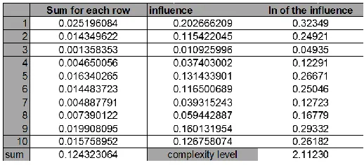
Finally, table showing the summation of each row, the influence of each operation in the system, and the natural logarithm (Ln) of the influence and the complexity level is provided below in Table XIV
TABLEXIV
NATURALLOGARITGMOFTEINFLUENCE
The level of complexity for the planned durations is approximately 1.375, meaning that the planned operation schedule is in a state of minor complexity level. The next step is to calculate the complexity for the actual operation schedule to compare between both plans and determine the next course of action.
2) Complexity calculation for actual operation
The level of complexity for the actual operation is 2.1123, representing a slight increase over the calculation of the planned operation. Here, a minor complexity level exists as well. Unfortunately, unlike the planned operation, there is a significant difference when comparing the influences of each step in both plans.
IV. ABC ANALYSIS
The complexity calculations for both the planned and actual operation models indicate that the 5th and 6th steps have the greatest influence on the system, i.e., nearly 36% each. We conducted an ABC analysis (Pareto Diagram) to prioritize and identify the most important sequences affecting the complexity calculation by comparing the influence levels. This will help management in tracking the most influential sequences in the operation plan.
A. Determining the Most Influential Sequence in the Operation Model
In this section, we present the Pareto diagrams starting with the planned operation schedule, followed by the actual operation schedule.
TABLE XV
CUMULATIVE INFLUENCE OF PLANNED OPERATION
The Table XV above illustrates that operations 6, 5, 8, 7, and 4 are the most influential sequences affecting the complexity
, and their cumulative influences amount to nearly 80%, meaning that if we can focus on these processes first and investigate the causes behind the delays occurring in these processes, we can eliminate 80% of the problem.
Unfortunately, analysis of the actual operational schedule indicated that there is a variance in the process.
TABLE XVI
CUMULATIVE INFLUENCE OF ACTUAL OPERATION
Table XVI illustrates that processes 1, 9, 5, 10, 6, 2, and 8 are the most influential sequences affecting the complexity. This means that a total of 7 processes affect the complexity in a severe way, in contrast to the planned operation, in which 5 processes are of particular interest.
V. CONCLUSIONS
When implementing the complexity for the planned and actual durations, no part mix ratio was available for the data, and the planned and actual durations resulted in minor complexity measurements. The levels of complexity for the planned and actual durations were 1.375 and 2.1123, respectively.
We also conducted an ABC analysis and found that some processes affected both plans:
Parts Repair (MRP) QEC Parts Rep Parts Purchasing Parts Repair Mod. Assembly
1. Complexity model:
The development of a static complexity measure can support managerial decisions on improving system operations. Hence, the proposed complexity measure is one in which both direct and indirect interactions are characterized by the form of influences. 2. Part mix ratio:
A part mix ratio should be determined and
implemented to reduce the complexity of the planned durations. Unfortunately, as noted above, when we spoke with SAEI engineers, they informed us that they had not established a part mix ratio because engine maintenance was not periodically
implemented. Thus, SAEI engineers should establish a part mix ratio for the engines and should implement it in the complexity measurement calculations to reduce the complexity level for both the actual and planned durations in a manner that will increase machine and man power utilization and thus reduce the delay time and cycle time.
3. A system should be implemented to follow up and inspect the workers to prevent delays. This system should be based on the planned durations after implementing the part mix ratio and reaching a suitable degree of complexity.
The productivity report should be resumed in the future because a measurable method to track progress in a quantitative manner is now available.
ACKNOWLEDGMENT
We would like to thank SAEI for providing us with the data. In addition, we like to thanks Eng. Mohammed hussain and Eng., Alhusan Naita for their data collections to carry out this work.
.REFERENCES
[1] Park, Kijung, and Gül E. Okudan Kremer.(2015) "Assessment of static complexity in design and manufacturing of a product family and its impact on manufacturing performance." International Journal of Production Economics 169 : 215-232.
[2] Weaver (1948) ,“Science and Complexity”, American Scientist, Vol. 36, pp. 536-544
[3] Yates (1978) , “Complexity and the limits to knowledge”, American Journal of Physiology - Regulatory, Integrative and Comparative Physiology, Vol.235, No.5, pp. R201-R204
[4] Allen and Torrens (2005) “Knowledge and complexity”, Futures, Vol.37, No.7, pp. 581-584.
[5] Serdar Asan, Seyda. (2009) "A methodology based on theory of constraints’ thinking processes for managing complexity in the supply chain."
[6] Perona, Marco, and Giovanni Miragliotta. (2004) "Complexity management and supply chain performance assessment. A field study and a conceptual framework." International journal of production economics 90 (1): 103-115.
[7] Deshmukh, A.V., Talavage, J.J., Barash, M.M., 1998, “Complexity in manufacturing systems- Part 1: Analysis of static complexity”, IIE Transactions, 30, (7) pp 645-655.