Modeling And Analysis Of A Closed Loop Supply Chain With Uncertain Lead Time In The Perspective Of Inventory Management

3643

Modeling And Analysis Of A Closed Loop Supply

Chain With Uncertain Lead Time In The

Perspective Of Inventory Management

Vipin Kumar Tyagi, Ruchi Goel, Manindar Singh, Sunil Kumar

Abstract : In the presented model an integrated inventory model with deterioration considering the two players is developed; the supplier and the retailer. Here the supplier consists the three shops for production, remanufacturing and for the collection of the returned items. Production rate is considered as demand dependent also the demand is considered as price dependent. Shortages are permitted and assumed to be partially backlogged. Lead time is also considered which is assumed to be uncertain. The model is investigated under the inflationary conditions.

Keywords : Deterioration, Remanufacturing, Supply Chain, Inflation, Uncertain Lead Time, Shortages ——————————  ——————————

I.

INTRODUCTION

The awareness regarding the environmental problems is increasing gradually among the society. Governments as well as consumers are now paying attention to the utilization of natural resources. Therefore, the companies are also taking a step toward the reverse logistics. In last few decades the researchers as well as practitioners have given a lot of consideration to the perception of remanufacturing or repairability, remanufacturing process or the reparability in supply chain modeling was firstly introduced by Schrady(1967). Dobos and Richter, (2004), presented the model and stated that a pure strategy gives more suitable solution rather than the mixed strategy. A reverse logistics model with the collection investment was introduced by Savaskan, et al. (2004). Teunter (2004), have developed a Lot-sizing model with product recovery. King et al. (2006), characterized the repairability as the improvement of the faults in any product and expressed that the worth of this product is inferior compared to the new ones and these repaired ones can be sold in any secondary market in the same condition. Chung et al. (2008), developed a reverse channel for the multi echelon supply chain system. Thereafter

Singh et al. (2013), have developed a

production/remanufacturing model with shortages using flexible rates. Currently Saxena et al. (2017) have presented a green supply chain model with vendor/buyer integration and Saxena et al. (2019) have investigated a studied the remanufacturing/production cycles with an alternative market. Banerjee (1986) has investigated a economic lot size model with the vender, buyer integration. In a subsequent study, Goyal and Nebebe (2000) have proposed a single vendor single buyer generalized model for integrated production policy. Hadidi, et al. (2011) have developed an integrated inventory model for production scheduling. After that Kumar et al. (2015) have presented their models along the same line of research using preservation technology and learning in supply chain. Recently Kumar, (2019) has proposed an production model for the

perishable items with seasonal effect and volume flexibility under the finite horizon. Yadav et al. (2019) have provided a deteriorating inventory model item under the effect of inflation. In the proposed article a closed loop supply chain inventory model for repairable items has been developed. It is assumed that the pre-owned items are gathered from the market and a specific proportion of these items is fixed and remanufactured. These items are conveyed to the retailer, for which an uncertain lead time is considered. The total average expense for the incorporated framework has been determined. The theoretical results have been verified with the help of a numerical illustration.

II.

A

SSUMPTION

1.The model is developed here for the integrated production of newly produced material and the remanufacturing of the buyback products.

2.The market demand is assumed to be price dependent.

3.The production is assumed to be the demand dependent.

4.The lead time is considered for the retailer.

5.Deterioration is taken into consideration.

6.Model is developed under the inflationary environment.

7.The shortages are permitted on the end of the retailer part which is assumed to be partially backlogged.

Notations:

α, β demand parameters

b collection parameter, b<1

θ deterioration rate

a production parameter, a≥1

p1, p2 selling price per unit for the producer and

the retailer

y the lead time

n number of replenishment cycles for the retailer

cR acquisition cost per unit

cm procurement cost per unit

sr remanufacturing cost per unit

sm production cost per unit

hr holding cost per unit for remanufactured

items

hm holding cost per unit for produced

items

hR holding cost per unit for collective items _________________

 Sunil Kumar (Corresponding Author) Department of Mathematics,

Swami Vivekanand Subharti University, Meerut. Email: gkv.sunil@gmail.com.

 Vipin Kumar Tyagi Department of Mathematics, SBAS Shobhit University, Meerut.

 Ruchi Goel Department of Mathematics, DN College, Meerut.

hs holding cost per unit for the retailer

O ordering cost per order

c1 production cost per unit

c4 deterioration cost per unit

c3 lost sale cost per unit

c2 shortage cost per unit

K1 set up cost for remanufacturing

process

K2 set up cost for fresh production

process

K3 set up cost for the collection process

η backlogging rate

r inflation rate

III.

M

ATHEMATICAL

M

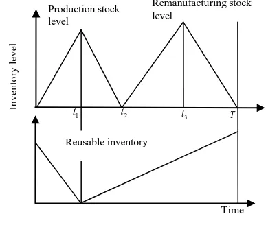
ODELING

The stock behavior of the reverse logistics system during the complete cycle is depicted in the following figure.

If the differential equations of the system are given as follow:

1 1

'( ) ( 1) ( ) 0

r r

I t p a I t  t t (1)

1 1 2

'( ) ( )

r r

I t  pI t t  t t (2)

1 2 3

'( ) ( 1) ( )

m m

I t p a I t t  t t (3)

1 3

'( ) ( )

m m

I t  pI t t  t T (4)

2 1

'( ) ( ) ( ) 0

R R

I t p ba I t  t t (5)

2 1

'( ) ( )

R R

I t b p I t t  t T (6) With boundary conditions:

2 2 1

(0) 0, ( ) 0, ( ) 0, ( ) 0, ( ) 0

r r m m R

I  I t  I t  I T  I t 

The solutions of above mentioned differential equations are given as follow:

1

1

( ) ( 1) (1 t) 0

r

p

I t a e t t

     

     (7)

2 ( ) 1

1 2

( ) ( t t 1)

r

p

I t e t t t

     

    (8)

2 ( ) 1

2 3

( ) ( 1) (1 t t )

m

p

I t a e t t t

     

     (9)

( ) 1

3

( ) ( T t 1)

m

p

I t e t t T

     

    (10)

1 ( ) 2

1

( ) ( ) (1 t t ) 0

R

p

I t b a e t t

     

     (11)

1 ( ) 2

1

( ) (1 t t )

R

b p

I t e t t T

     

    (12)

The behavior of the retailer’s inventory is shown in fig 2. Here we have assumed that the retailer places his order at time zero and receives the inventory at time t=y, where y is the lead time. During this period when the retailer does not have the inventory, he bears the shortages which are assumed to be fully backlogged. During [y, T1] inventory level depletes because of

the demand and deterioration. At t= T1, the inventory level

becomes zero.

The governing equations to depict the stock behavior of the retailer are given as follow:

2

'( ) 0

s

I t  p  t y (13)

2 1

'( ) ( )

s s

I t I t  p y t T (14)

With boundary condition Is(0)0 and (0)Is 0

The solutions of the above equations are given by: 2

( ) 0

s

I t  pt  t y (15)  



1



2

1

( ) 1 T t

s

p

I t e y t T

     

    (16)

Where T₁ T n



Cost component at the manufacturer’s end are given as follows:

Procurement and acquisition cost =

3

2 1 0

t T

rt rt

m R

t

a

c e dt c Re dt

p

  _ 





Production and remanufacturing cost

=

3 1

2 1 0 1

t t

rt rt

m R

t

a a

S e dt S e dt

p p

  _  





Holding cost 1 2 1 3 1

2 3 1

0 0 [ ( ) ( ) ] [ ( ) ( ) ] [ ( ) ( ) ] t t rt rt

r r r

t

t T t T

rt rt rt rt

m m m R R R

t t t

h I t e dt I t e dt

h I t e dt I t e dt h I t e dt I t e dt

          













Production stock level Time T 3 t 2 t 1 t Remanufacturing stock level In v e n to ry l e v e l Reusable inventory

Fig. 1: Stock behaviour of the reverse logistics inventory model

3645 Set up cost = K₁K₂K₃

Salvage cost = S bR (1 )p₂ T



 _ 

Hence the total cost for the manufacturer is

TCm = 1

T [Set up cost + Holding cost +Procurement cost +

Acquisition cost + Manufacturing cost + Remanufacturing cost +

Salvage cost]

Cost component at the retailer’s end are given as follows: Ordering cost= O

Purchasing cost =



Is( )y q c



1

Where 2

T n

v

q



pdt

Holding cost= ( ) v

rt s s

y

h



I t e dt

Shortage cost = 2 2

T n

rt

v

c



pe dt

Lost sale cost= 3 2 (1 )

T n

rt

v

c



p e dt

Deterioration cost= 4 ( ) 2

T n

s y

c I y pdt

   _      





Total cost for the retailer is given by: TCs =

n

T [Ordering cost + Deterioration cost + Purchasing cost

+ Holding cost + Shortage cost + Lost sale cost]

Hence the total average expense of the system per unit time of the given inventory model as a function of t1, t2, t3, v, y and T say

T.C. (t1, t2, t3, v, y, T) is given by

T.C. =

1 2 1

2 3 3

1

3 2 3 2 1

1 1 1 1

( )

1 1 2

1 1 ( ) ( ) 3 2 1 1 3 1 1 1 1 [ ( ) ( ) 1 1

{( 1) ( ) ( )}

1 1

{( 1) (( ) ) (

( ) 1

( ))} { ( )

m R m r

t t t

r

t t T t

m

t

R

a b a a

t t c Tc s t t s t

T p p p p

e e

h a t t t

p p

e e

h a t t

p p

b a e b

T t h t

p p                                                                   1 1 ( )

1 2 3

2 (1 ) 1 2 2 (1 ) 2 2 2 (1 ) 3 4

2 2 2

(( )

1

( 1)} {(1 ) } ]

{ ( ( 1) ( ))

( 1)

( ( 1)) ( )

(1 )( ) ( ( 1) ( ))}

t T av y y s y T t

e K K K s b T

p

n T

c e y

T p p n

e T

h y O c y

p p n

T T

c y c e y

p n p p n

                 _{ }       _                                  ( 17)

From equation (17) it is observed that the total annual cost is the function of the variables t1, t2, t3, y and T. Hence to minimize

the total annual cost, we have to optimize the values of t1, t2, t3, y

and T.

Using the boundary conditions, we get some relations between the variables such as follows.

1 2 1

2 3 3

1 1

( )

( ) ( )

( )

( 1)(1 ) ( 1)

( 1)(1 ) ( 1)

( )(1 ) (1 )

t t t

t t T t

t t T

a e e

a e e

b a e b e

                      

IV.

N

UMERICAL ANALYSIS

The theoretical results are illustrated through the numerical example with the help of the software Mathematica 8.0 The input values are given below in appropriate units:

1 2

1 2 3

1

1500 , 25 , 30 , 1.25, 0.75, 0.45,

0.85, 5, 2.5, 0.45 / , 0.45 / ,

0.3 / , 0.01, 12 / , 8 / ,

11.5 / , 1000 , 1200 , 1500 ,

30 /

r m

R m R

av

units p Rs p Rs a

b n h Rs unit h Rs unit

h Rs unit c Rs unit c Rs unit

s Rs unit K Rs K Rs K Rs

c Rs unit

                       

 2 3 4

3 3

, 4 / , 5 / , 30 / ,

5 / , 0.4 / , 0.6, 500 / , 0.04

c Rs unit c Rs unit c Rs unit

c Rs unit h Rs unit O Rs order r

  

    

Using the above parametric values and the solution procedure provided in the previous section, we have obtained the computational results. The optimal values are presented in the Table 1.

Table 1: optimal results of the given reverse logistics system.

t1 t2 t3 T T1 Y TC

2 4

6 8

10 20

40 60

80 100

550 600 650 700

2 4

6 8

10

Fig 3: Convexity of the total cost function

Sensitivity analysis:

To study the effect of the variation of the input parameters on optimal solution, a sensitivity analysis has been performed which is shown in the Tables 2 (Appendix). And the effect of the different parameter on the total cost is shown in the figures 4-12.

Fig 4: T.A.C. v/s α

Fig. 5: T.A.C. v/s p1

Fig. 6: T.A.C. v/s a

Fig. 7: T.A.C. v/s γ

3647

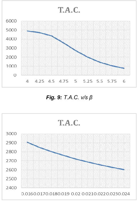
Fig. 9: T.A.C. v/s β

Fig. 10: T.A.C. v/s θ

Fig. 11: T.A.C. v/s hs

Concluding remarks:

1. From the table 2, we have seen that absolute normal expense(TC) and cycle length T are emphatically delicate to the adjustments sought after parameter α1 and negative touchy to

the adjustments in selling cost p1.

2. It is plainly noticeable that with the addition underway parameter (a), the process duration T increments and TC of the framework shows the switch impact and with the augmentation in parameter γ, the process duration stays steady and TC diminishes somewhat.

3. Table 2 shows the impact of changes in returned parameter b, it is seen that with the addition in parameter b, the process duration T somewhat diminishes and TC of the framework increments.

4. We have seen that with the augmentation sought after parameter β and decay rate θ, the process duration T increments and TC diminishes.

5. It is observed that with the addition in holding cost hs, the

process duration T builds somewhat and TC diminishes constantly.

CONCLUSION

In this paper a coordinated stock model for reparability/remanufacturing has been created. The Production rate is thought to be a component of demand rate. The lead time is additionally considered for the retailer. Here the provider comprises the three shops for production, remanufacturing and for the assortment of the returned things. Shortages are allowed and thought to be partially backlogged. The model is examined under the inflationary conditions. The hypothetical outcomes are outlined with the assistance of a numerical model. Affectability examination regarding diverse framework parameters is likewise talked about to check the strength of the model. This model further can be reached out for impreciseness and impact of learning.

REFERENCES

[1] Banerjee A. (1986), A joint economic-lot-size model for purchaser and vendor, Decision Science, 17, 292–311. [2] Chung S. L., Wee H. M. and Yang P. C. (2008), Optimal

policy for a closed-loop supply chain inventory system with remanufacturing, Mathematical and Computer Modeling, 48, 867–881.

[3] Dobos, I., Richter, K., (2004). An extended production/recycling model with stationary demand and return rates. International Journal of Production Economics 90, 311–323.

[4] Goyal, S. K. and Nebebe, F. (2000). Determination of economic production-shipment policy for a single-vendor single-buyer system. European journal of operational research, 121, 175–178.

[5] Hadidi, L.A., Turki, U.M.A. and Rahim, M.A. (2011) ‘An integrated cost model for production scheduling and perfect maintenance’, Int. J. of Mathematics in Operational Research, Vol. 3,No. 4, pp.395–413.

[6] King A. M., Burgess S. C., Ijomah W. and McMahon C. A. (2006), Reducing waste: Repair, recondition, remanufacture or recycle?, Sustainable Development, 14(4), , 257-267.

[7] Kumar, J., Tanwar, A., Kumar, S., Rana, A.K., Saxena, N. (2019). An EPQ deteriorating inventory model for seasonal products with volume flexibility under finite horizon. Journal of Advanced Research in Dynamical and Control Systems 11(6 Special Issue), 108-119.

learning in supply chain. Cogent Engineering, 2(1), 1045221.

[9] Savaskan R. C., Bhattacharya S. and Van Wassenhove L. N., Closed-loop supply chain models with product remanufacturing, Management Science, 50 (2), (2004), 239–252.

[10]Saxena, N., Sarkar, B., & Singh, S. R. (in press). Selection of remanufacturing/production cycles with an alternative market: a perspective on waste management. Journal of

Cleaner Production, 118935.

DOI:https://doi.org/10.1016/j.jclepro.2019.118935

[11]Saxena, N., Singh, S. R., & Sana, S. S. (2017). A green supply chain model of vendor and buyer for remanufacturing. RAIRO-Operations Research, 51(4), 1133-1150.

[12]Schrady D. A. (1967), A deterministic Inventory model for repairable items, Naval Research Logistics Quarterly, 14(3), 391–398.

[13]Singh S. R., Prasher L. and Saxena N. (2013), A centralized reverse channel structure with flexible manufacturing under the stock out situation, International Journal of Industrial Engineering Computations,4,559-570. [14]Teunter, R.H. (2004). Lot-sizing for inventory systems with

product recovery. Computers and Industrial Engineering 46 (3), 431–441.

[15]Yadav, A.S., Bansal, K.K., Kumar, J., Kumar, S. (2019). Supply chain inventory model for deteriorating item with warehouse & distribution centers under inflation. International Journal of Engineering and Advanced Technology. 8(2), pp. 7-13.

[16]Tyagi, V. K., Goel, R., Singh, M., Kumar, S., (2019). A Supply Chain Inventory Model for Deteriorating Items with Variable Lead Time and Varying Demand under Shortages. Jour of Adv Research in Dynamical & Control Systems, Vol. 11(6), 87-96.

APPENDIX

Table 2: The effect of the variation in the different parameters:

Variation in

percentage T T1

y

TC

Variation with respect to α

-20% 28.27125 5.65425 1.88475 2600.345

-15% 28.35538 5.671076 1.890359 2630.725

-10% 28.43738 5.687476 1.895825 2661.115

-5% 28.517 5.7034 1.901133 2691.52

0% 28.5945 5.7189 1.9063 2721.945

5% 28.67 5.734 1.911333 2752.38

10% 28.7435 5.7487 1.916233 2782.835

15% 28.81513 5.763026 1.921009 2813.3

20% 28.88488 5.776976 1.925659 2843.78

Variation with respect to p1

-20% 29.54463 5.908926 1.969642 3178.03

-15% 29.26988 5.853976 1.951325 3027.705

-10% 29.021 5.8042 1.934733 2905.605

-5% 28.7965 5.7593 1.919767 2805.265

0% 28.5945 5.7189 1.9063 2721.945

5% 28.41325 5.68265 1.894217 2652.1

10% 28.25063 5.650126 1.883375 2593.05

15% 28.10475 5.62095 1.87365 2542.74

20% 27.97388 5.594776 1.864925 2499.575

Variation with respect toa

-20% 24.19638 4.839276 1.613092 3103.985

-15% 25.3695 5.0739 1.6913 2988.865

-10% 26.49413 5.298826 1.766275 2888.23

-5% 27.5695 5.5139 1.837967 2799.85

0% 28.5945 5.7189 1.9063 2721.945

5% 29.5685 5.9137 1.971233 2653.065

3649

15% 31.3615 6.2723 2.090767 2537.835

20% 32.18013 6.436026 2.145342 2489.68

Variation with respect to γ

-20% 28.5945 5.7189 1.9063 2732.29

-15% 28.5945 5.7189 1.9063 2729.735

-10% 28.5945 5.7189 1.9063 2727.12

-5% 28.5945 5.7189 1.9063 2724.53

0% 28.5945 5.7189 1.9063 2721.945

5% 28.5945 5.7189 1.9063 2719.36

10% 28.5945 5.7189 1.9063 2716.77

15% 28.5945 5.7189 1.9063 2714.185

20% 28.5945 5.7189 1.9063 2711.6

Variation with respect tob

-20% 29.36063 5.872126 1.957375 2665.815

-15% 29.16275 5.83255 1.944183 2680.035

-10% 28.96913 5.793826 1.931275 2694.125

-5% 28.77988 5.755976 1.918659 2708.095

0% 28.5945 5.7189 1.9063 2721.945

5% 28.41313 5.682626 1.894209 2735.675

10% 28.23563 5.647126 1.882375 2749.285

15% 28.06163 5.612326 1.870775 2762.785

20% 27.89125 5.57825 1.859417 2776.17

Variation with respect to β

-20% 9.663763 1.932753 0.644251 4889.24

-15% 12.03595 2.40719 0.802397 4729.62

-10% 15.58138 3.116276 1.038759 4370.14

-5% 20.85475 4.17095 1.390317 3567.84

0% 28.57088 5.714176 1.904725 2721.945

5% 39.71925 7.94385 2.64795 2002.305

10% 55.29013 11.05803 3.686009 1450.17

15% 76.46588 15.29318 5.097725 1048.75

20% 104.4886 20.89772 6.965907 763.995

Variation with respect to θ

-20% 28.09125 5.61825 1.87275 2905.925

-15% 28.16563 5.633126 1.877709 2850.42

-10% 28.28213 5.656426 1.885475 2802.165

-5% 28.42813 5.685626 1.895209 2759.7

0% 28.5945 5.7189 1.9063 2721.945

5% 28.77463 5.754926 1.918309 2688.065

10% 28.96338 5.792676 1.930892 2657.43

15% 29.15713 5.831426 1.943809 2629.545

20% 29.353 5.8706 1.956867 2604.01

Variation with respect to hs

-20% 28.55275 5.71055 1.903517 2809.75

-15% 28.56313 5.712626 1.904209 2785.74

-10% 28.57363 5.714726 1.904909 2763.19

-5% 28.58413 5.716826 1.905609 2741.96

0% 28.5945 5.7189 1.9063 2721.945

5% 28.605 5.721 1.907 2703.045

15% 28.626 5.7252 1.9084 2668.225