OPTIMIZATION AS AN ANALYSIS TOOL FOR HUMAN
COMPLEX PROBLEM SOLVING*
SEBASTIAN SAGER†, CAROLA M. BARTH‡, HOLGER DIEDAM§
, MICHAEL ENGELHART§,
ANDJOACHIM FUNKE‡
Abstract.We present a problem class of mixed-integer nonlinear programs (MINLPs) with nonconvex continuous relaxations which stem from economic test scenarios that are used in the analysis of human complex problem solving. In a round-based scenario participants hold an executive function. A posteriori a performance indicator is calculated and correlated to personal measures such as intelligence, working memory, or emotion regulation. Altogether, we investigate 2088 optimization problems that differ in size and initial conditions, based on real-world experimental data from 12 rounds of 174 participants. The goals are twofold. First, from the optimal solutions we gain additional insight into a complex system, which facilitates the analysis of a participant’s performance in the test. Second, we propose a methodology to automatize this process by provid-ing a new criterion based on the solution of a series of optimization problems. By providprovid-ing a mathematical optimization model and this methodology, we disprove the assumption that the“fruit fly of complex problem solving,”theTailorshopscenario that has been used for dozens of published studies, is not mathematically accessible—although it turns out to be extremely challenging even for advanced state-of-the-art global opti-mization algorithms and we were not able to solve all instances to global optimality in reasonable time in this study. The publicly available computational tool Tobago [TOBAGO web site https://sourceforge.net/ projects/tobago] can be used to automatically generate problem instances of various complexity, contains in-terfaces toAMPLandGAMS, and is hence ideally suited as a testbed for different kinds of algorithms and solvers. Computational practice is reported with respect to the influence of integer variables, problem dimen-sion, and local versus global optimization with different optimization codes.
Key words. mixed-integer programming, nonlinear programming, cognitive psychology, measurement and performance
AMS subject classifications.90C11, 90C30, 91E10, 91E45
DOI.10.1137/11082018X
1. Introduction. The methodologyoptimization has a long record of successful improvements in many technological and scientific areas, being used for tasks such as design, scheduling, business control rules, process control, and the like. More recently, optimization has also been successfully applied in the context of inverse problems, e.g., for the choice and calibration of mathematical models or as a modeling paradigm for biological systems. In this work we propose to use numerical optimization as an analysis tool for the understanding of human problem solving, which to our knowledge has not yet received much attention.
Complex problem solving is defined as ahigh-order cognitive process. The complex-ity may result from one or several different characteristics, such as a coupling of sub-systems, nonlinearities, dynamic changes, intransparency, or others [16]. The main
*Received by the editors January 6, 2011; accepted for publication (in revised form) June 24, 2011; pub-lished electronically September 20, 2011. Financial support was provided by the Heidelberg Graduate School
Mathematical and Computational Methods for the Sciencesand of the Postgraduate Fellowship Program of the state of Baden-Württemberg.
http://www.siam.org/journals/siopt/21-3/82018.html
†Corresponding author. Interdisciplinary Center for Scientific Computing (IWR), Heidelberg University,
69120 Heidelberg, Germany ([email protected]).
‡Department of Psychology, Heidelberg University, 69117 Heidelberg, Germany (carola.barth@psychologie
.uni-heidelberg.de, [email protected]).
§
intention of the research fieldcomplex problem solvingof human beings is the desire to understand how certainvariablesinfluence a solution process. In generalpersonal and
situational variablesare differentiated. The most typical and frequently analyzed
per-sonal variable isintelligence. It is an ongoing debate how intelligence influences complex problem solving [53]. Other interesting personal variables are working memory [43],
amount of knowledge [34], andemotion regulation [40]. Situational variables like the
impact of goal specificity and observation [39], feedback [12], and time constraints
[26] attracted less attention.
Psychologists have been working in the research fields of problem solving for ap-proximately 80 years. One of the groundbreaking works by Ewert and Lambert in 1932 [17] was based on the disk problem, more commonly known as theTower of Hanoi. Since the 1970s and 1980s computer-based test scenarios have also been used, e.g., LEARN [28], Moro [46], FSYS 2.0 [51], andTailorshop, which is the basis for this study.
Tailorshopis sometimes referred to as the“Drosophila”for problem solving researchers
[24] and thus a prominent example for a computer-based test scenario. All mentio-ned scenarios try to reflect the characteristics of real-life problems by simulating a microworld [27].
The overall idea, compared to early works in problem solving, is still the same: one evaluates the performance of a participant by calculating an indicator function and either correlates it to personal attributes, such as the intelligence quotient [32], or ana-lyzes the influence of different experimental conditions for groups of participants [4]. The main difference is that for the early test scenarios the correct solution is known at every stage. For more complex scenarios the performance evaluation is not so straightforward. In this paper we address the question of how to get a reliable performance indicator for theTailorshopscenario.Tailorshophas been used in a large number of studies, e.g., [42], [35], [33], [37], [4], [5]. Also comprehensive reviews on studies and results in con-nection withTailorshophave been published; see [20], [22], [23], [25], [24], in which more information on the psychological background can be found.
InTailorshopparticipants make economic decisions to maximize the overall balance
propose to compare the decisions to mathematically optimal solutions. For a recent re-view onTailorshop success criteria, see [15].
Because all previously used indicators have unknown reliability and validity, we propose to compare the decisions to mathematically optimal solutions. Hussy [31, p. 62] writes in 19851
“Only when it will be possible, e.g., by means of mathematical optimization meth-ods, to determine the objectively optimal solution process to compare the process chosen by the proband with it, will this severe problem be overcome.”
The availability of an objective performance indicator is an obstacle for analysis, and it has often been argued that inconsistent findings are due to the fact that
“: : : it is impossible to derive valid indicators of problem solving performance for tasks that are not formally tractable and thus do not possess a mathematically optimal solution. Indeed, when different dependent measures are used in studies using the same scenario (i.e., Tailorshop [21], [47], [41]), then the conclusions frequently differ” as stated by Wenke and Frensch [52, p. 95]. Based on a mathematical model of the
Tailorshop, an optimization is performed for every round of the participant’s data,
start-ing with exactly the same conditions as the participant. By comparstart-ing these optimal values that indicatehow much is still possibleif all future decisions were made perfectly, an analysis of at what rounds potential has been lost by decisions can be obtained. Based on optimization theory, even further insight into what decisions were decisive for bad or good performance can be obtained by analyzing Lagrange multipliers.
To our knowledge, numerical optimization methods have only scarcely been used for the analysis of participants’ decisions in complex environments like Tailorshop. Cognitive psychologists and economists have been using simulation methods for finding optimal solutions for simple tasks within strongly constrained environments. Also, in the context ofexperimental economicsstudies have been performed, however, to our knowl-edge not with explicit mathematical representations of the scenarios, including nonli-nearities and integer variables. The general approach to compare performance to optimal solutions has been discussed by [36]. However, the authors do not provide a mathematical model for their test scenarioEPEX. Hence, they need to use the software as a black box for brute-force simulation or derivative free strategies, such as Nelder– Mead [38], or genetic algorithms. Such strategies result in significantly higher computa-tional runtimes, give less insight, and have poor theoretical convergence properties. Our approach formulates the simulation task as equality constraints of the optimization pro-blem and thus allows us to apply modern optimization techniques, including simulta-neous strategies that solve simulation and optimization tasks at the same time. They have shown to be superior in many cases; compare, e.g., [8], [7], [2].
It turns out that the optimization problems that need to be solved in the context of
theTailorshopscenario are mixed-integer nonlinear programs with nonconvex
contin-uous relaxations. Whenever optimization problems involve variables of contincontin-uous and discrete nature, the term mixed-integer is used. In our case they can be interpreted as discretized optimal control problems. See [44] for a recent review of algorithms to treat continuous-time mixed-integer optimal control problems. However, as the time grid is fixed, the applicability of such methods is limited, and we focus on combinatorial methods.
1
Progress in mixed-integer linear programming (MILP) started with the fundamen-tal work of Dantzig and coworkers on the Traveling Salesman problem in the 1950s. Since then, enormous progress has been made in areas such as linear programming
(and especially in thedual simplexmethod that is the core of almost all MILP solvers because of its restart capabilities), in the understanding ofbranching rulesand more powerful selection criteria such as strong branching, the derivation of tight cutting
planes, novelpreprocessingandbound tightening procedures, and of course the
compu-tational advances roughly following Moore’s law. For specific problem classes problems with millions of integer variables can now be routinely solved [3]. Also, generic problems can often be solved very efficiently in practice, despite the known exponential complex-ity from a theoretical point of view [9].
The situation is different in the field of mixed-integer nonlinear programming (MINLP). Only at first sight many properties of MILP seem to carry over to the non-linear case. Restarting nonnon-linear continuous relaxations within branching trees is essen-tially more difficult than restarting linear relaxations (which, e.g., BARON and
Couennealso use for nonlinear problems), as no dual algorithm comparable to the dual
simplex is available in the general case. Nonconvexities lead to local minima and do not allow for easy calculation of subtrees, which is important to avoid an explicit enumera-tion. Additionally, nonlinear solvers are slower and less robust than LP solvers. How-ever, the last decade saw great progress triggered by cross-disciplinary work of integer and nonlinear optimizers, resulting in generic MINLP solvers, e.g., [1], [10]. Most of them, however, still require the underlying functions to be convex. Comprehensive sur-veys on algorithms and software for convex MINLPs are given in [29], [11]. Recent pro-gress in the solution of nonconvex MINLPs is in most cases based on methods from global optimization, in particular convex under- and overestimation. See, e.g., [18], [48] for references on general under- and overestimation of functions and sets.
Our intention is to foster interdisciplinary research between psychologists and ap-plied mathematicians. We provide the research community in the field of complex pro-blem solving with the open source software toolTobago[45]. This data generation and analysis tool can be hooked to a variety of optimization solvers. Currently the software supportsAMPL[19] andGAMS[14] interfaces. This allows for the usage of solvers from
theCOIN-ORinitiative, which are also available under a public license. In this study we
used the global solversCouenne[6] and the local solversBonmin[10] andIpopt[50]. In addition, we ran the global solverBARON[49] on the NEOS server.
It turns out, however, that the size and complexity of the problems presented in this paper lead to extremely long runtimes of the global solvers and can only be used on a small subset of the problems. We present a problem-specific lower bound to avoid bad local maxima and guarantee monotonicity of the analysis function that builds on the locally optimal objective function values. However, additional future work in several mathematical areas will be needed to address all demands of researchers incomplex
pro-blem solving.
[22], [23], [25], [24]), in which more information on the psychological background can also be found.
A participant has to take economic decisions to maximize the overall balance of a small company specialized in the production and sales of shirts. The scenario comprises 12 rounds (months), in which the participant can modify infrastructure (employees, ma-chines, distribution vans), financial settings (wages, maintenance, prices), and logistical decisions (shop location, buying raw material). As feedback he gets some key indicators in the next round, such as the current number of sold shirts, machines, employees, and the like. Arrows next to the indicators show if the value increased or decreased with respect to the previous round.
There are two different kinds of machines to produce either 50 or 100 shirts per month. Workers need to specialize for work on either one of them. The machines need to be maintained and equipped with raw material to actually produce something. The possible production depends furthermore on the satisfaction of the workers, linked to the controls wages and social expenses. Vans influence the demand in a positive way. Furthermore, advertisement, location of the sales shop, and shirt pricing decisions can be used to maximize profit.
We derive a mathematical formulation as an optimization problem. The basic idea is that for different initial values (the current state in roundnsof a participant’s test run) the optimal solution for the remainingN−ns rounds can be calculated. The optimal solution can then either be used for a manual comparison and analysis of the participant’s decisions, section 3, or for an automated indicator function, as discussed in section 4.
TheTailorshopwas developed as a computer-based test scenario inGW-Basiccode
in the early 1980s. This implementation was the starting point for the mathematical modeling process. Figure A.1 in the appendix shows a short extract of this file. The scenario as it is implemented inGW-Basichas several shortcomings and assumptions one might disagree with. However, this implementation and similar ones have been used over years, and at the point where interdisciplinary cooperation started, most of the data of the 174 participants had already been evaluated in a cumbersome procedure. Hence the formulation of test scenarios that have better mathematical properties has been postponed to future work, and the mathematical model which we derive from the
GW-Basiccode can be considered as given, even if it is not in all aspects close to reality.
On the basis of theGW-Basiccode we derived a mathematical optimization pro-blem for a participant and month0≤ns<N as
max x;u;sFðxNÞ
s:t:xkþ1¼Gðxk; uk; sk; pÞ; k¼ns: : : N−1; 0≤Hðxk; xkþ1; uk; sk; pÞ; k¼ns: : : N−1;
uk∈Ω; k¼ns: : : N−1;
xns¼xp ns:
ð2:1Þ
min–max expressions by standard techniques using the constraints (2.27)–(2.31). For details on these and further reformulations, see section A.2.2. We define
ðxp; upÞ ¼ ðxp
0; : : : ; xpN; up0; : : : ; upN−1Þ
to be the vector of decisions and state variables for all months of a participant. Certain entries xpns enter (2.1) as fixed initial values. Participant independent initial values xp0 ¼px0 are given alongside fixed parameterspin Table A.1 in the appendix. Random valuesξappear in the equations, e.g., line 2810 in Figure A.1. However, a detailed ana-lysis of the compiled code revealed that the random values are only dependent on an initialization (seed) within theGW-Basiccode; hence they are identical for all parti-cipants and can be fixed in the optimization problem. See Table A.2 in the appendix. The goal is to find decisionsuk that maximize the overall balance at the end of the time horizon. The objective function is given by
FðxNÞ ¼xOBN :
Whenever we use the expressionrelaxed optimization problemthis will refer to the case in which the sets of points in (2.21)–(2.24) are replaced by their convex hulls. The state propagation lawGð·Þis determined by the following set of equations for all k∈f0; : : : ;11g. For the sake of readability we omit the implicitly given units in the equations.
The number of machines for 50 and 100 shirts per month depends on buying and selling of machines. Note that there is a difference between buying and selling in the base capital equation so that two independent controls are needed here:
xM50
kþ1 ¼xMk 50þukΔM50−uδkM50;
ð2:2Þ
xM100
kþ1 ¼xMk 100þukΔM100−uδkM100:
ð2:3Þ
TABLE2.1
Controls and states in theTailorshopoptimization problem withk∈f0; : : : ;11gfor controls, respectively,
k∈f0; : : : ;12gfor states. Note that units are only given implicitly in the test scenario.
Decision uk unit1 State xk unit1
advertisement uADk MU machines 50 xM50
k machines
shirt price uSPk MU machines 100 xM100
k machines
buy raw material uΔkMS shirts workers 50 xW50
k workers
workers 50 uΔkW50 workers workers 100 xW100
k workers
workers 100 uΔkW100 workers demand xDEk shirts
buy machines 50 uΔkM50 machines vans xVAk vans
buy machines 100 uΔkM100 machines shirts sales xSSk shirts
sell machines 50 uδkM50 machines shirts stock xSTk shirts
sell machines 100 uδkM100 machines possible production xPPk shirts
maintenance uMAk MU actual production xAPk shirts
wages uWAk MU material stock xMSk shirts
social expenses uSCk MU satisfaction xSAk —
buy vans uΔkVA vans machine capacity xMCk shirts
sell vans uδkVA vans base capital xBCk MU
choose site uCSk — capital after interest xCAk MU
overall balance xOBk MU
For the workers a single control which stands for hiring and firing workers is suffi-cient since there is no such difference (one might even avoid the state variable if the control was the current number of workers, but we stick to the hiring control for histor-ical reasons):
xW50
kþ1 ¼xWk 50 þuΔkW50;
ð2:4Þ
xW100
kþ1 ¼xWk 100 þuΔkW100:
ð2:5Þ
Demand depends on a time dependent parameterpDEk as well as on the advertise-ment expenses and the number of vans multiplied by a factor depending on the site, f1ðuCS
k Þ(see section A.2.1),
xDE
kþ1¼100pDEk −50þ
uAD
k
5 þ100ðxVAk þukΔVA−uδkVAÞ
f1ðuCS
k Þ:
ð2:6Þ
While the influence of advertisement is bounded (see below and section A.2.2) the effect of vans is unbounded. This leads to unboundedness of the whole problem. In sec-tion A.2.2 our approach to generate reasonable solusec-tions anyway is described.
For the vans again, two controls for buying and selling are needed due to differences in the base capital. Shirt sales are determined by the slack variablesSSk , and shirts in stock depend on the slack variables for actual productionsPPk and shirt salessSSk ,
xVA
kþ1¼xVAk þukΔVA−uδkVA;
ð2:7Þ
xSS
kþ1¼sSSk ;
ð2:8Þ
xST
kþ1¼xSTk þsPPk −sSSk :
ð2:9Þ
In the possible production equation, the part representing machine and worker de-pendence consists of a term for each machine type with slack variablessM50
k andsMk 100,
which are used to replace min expressions of workers and machines, multiplied by a machine capacity term (machines for 100 shirts have double machine capacity). This part is multiplied by the square root of workers’ satisfaction. The actual production is determined by a slack variable.
xPP
kþ1¼ ðsMk 50ðxMCk þ4pPk50 −2Þ þsMk100ð2xkMCþ6pPk100 −3ÞÞ
·
1 2þ
uWA
k −850
550 þ
uSC k 800
1 2 ;
ð2:10Þ
xAP kþ1¼sPPk .
ð2:11Þ
Raw material in stock depends on the use of material represented by the slack vari-able for actual production and the purchase of new material. Wages and social expenses influence satisfaction, and the machine capacity is determined by a slack variable:
xMS
kþ1¼xMSk þuΔkMS−sPPk ;
xSA
kþ1¼12þu WA
k −850
550 þ
uSC k 800; ð2:13Þ
xMC kþ1¼sMCk :
ð2:14Þ
The equation for base capital, xBC
kþ1¼xCAk þsSSk ·uSPk −pPRk ·ukΔMS−10000ukΔM50−f2ðuCSk Þ
þ8000xMCk
pMMuδkM50−20000uΔkM100þ16000x MC k
pMMuδkM100
−uAD
k −uMAk −ðxkW50þuΔkW50 þxkW100þuΔkW100Þ·ðuWAk þuSCk Þ
−2sPP
k −12ðxMSk þuΔkMS−sPPk Þ−xSTk −10000·uΔkVA
þ ð8000−100kÞ·uδkVA−500ðxVAk þuΔkVA−uδkVAÞ;
ð2:15Þ
contains all income and expenses during a round added to the capital after interest from the previous round. The income consists of the amount of shirts sold times the shirt price sSS
k ·uSPk , the sale of machines 8000ðxkMC∕ pMMÞukδM50 and16000ðxMCk ∕ pMMÞuδkM100
(de-pending on the current machine capacity), and the sale of vansð8000−100kÞ·uδkVA. Money is spent for the raw material bought times the price of a raw material unit
−pPR
k ·uΔkMS, the purchase of machines−10000ukΔM50 and−20000uΔkM100, the purchase of
vans −10000uΔkVA, advertisement and maintenance−uADk −uMAk , and the number of workers times wages plus social expenses −ðxW50
k þuΔkW50þxWk 100þuΔkW100Þ·ðuWAk þ
uSC
k Þ. Additionally, each unit of material in stock at the end of a round costs half a money
unit (MU) −1∕ 2ðxMSk þukΔMS−sPPk Þ, the production of a shirt costs two MU −2sPPk , each shirt in stock costs one MU, and each van costs 500 MU per round−500ðxVAk þ uΔVA
k −uδkVAÞ. There is another amount of money to be paid, which depends on the site,
−f2ðuCS
k Þ(see section A.2.2).
From the base capital, the capital after interest is computed by multiplying it with an interest rate factorð1þpIRÞ. Overall balance, the objective function, beside capital after interest, contains terms for material and shirts in stock, for machines, and for vans. However, machines are worth less in the overall balance than if they were sold:
xCA
kþ1¼xBCkþ1ð1þpIRÞ;
ð2:16Þ
xOB kþ1 ¼x
MC k
pMMð8000ðxkM50þuΔkM50−ukδM50Þ þ16000ðxMk100 þuΔkM100−uδkM100ÞÞ
þ ð8000−100kÞ·ðxVAk þuΔkVA−uδkVAÞ
þ2ðxMS
k þuΔkMS−sPPk Þ þ20ðxSTk þsPPk −sSSk Þ þxCAk .
ð2:17Þ
The feasible set of controls is defined by the following properties for all k∈f0; : : : ;11g:
uAD
k ∈½0;10000; uSPk ∈½10;100;
ð2:18Þ
uΔMS
k ∈½0;50000; uMAk ∈½0.1;100000;
uWA
k ∈½850;5000; uSCk ∈½0;10000;
ð2:20Þ
uΔW50
k ∈f−200;−199; : : : ;200g; ukΔW100 ∈f−200;−199; : : : ;200g;
ð2:21Þ
uΔM50
k ∈f0;1; : : : ;200g; ukΔM100 ∈f0;1; : : : ;200g;
ð2:22Þ
uδM50
k ∈f0;1; : : : ;200g; ukδM100 ∈f0;1; : : : ;200g;
ð2:23Þ
uCS
k ∈f0;1;2g:
ð2:24Þ
Furthermore, for allk∈f0; : : : ;11gthe constraints uΔW50
k ≥ −xWk 50; ukΔW100 ≥ −xWk 100;
ð2:25Þ
uδM50
k ≤xMk 50; ukδM100 ≤xMk100
ð2:26Þ
need to hold. Slack variables are used to reformulate min expressions (see also section A.2.2), and the bounds on the slack variables read as
sPP
k ≤xMSk þuΔkMS; sPPk ≤xPPkþ1;
ð2:27Þ
sMC
k ≤pMM; sMCk ≤0.9xMCk þ0.017 u MA k
xM50
kþ1þ10−8xkMþ1001 þ10−8
;
ð2:28Þ
sSS
k ≤xSTk þxAPkþ1; sSSk ≤54
xDE
k
2 þ280
·2.7181− uSP2
k 4250;
ð2:29Þ
sM50
k ≤xWkþ501; skM50 ≤xMkþ501;
ð2:30Þ
sM100
k ≤xWkþ1001 ; skM100 ≤xMkþ1001
ð2:31Þ
for allk∈f0; : : : ;11g.sPPk is used for the minimum of possible production and material in stock. WithsMCk , the minimum of maximum machine capacitypMMand the machine capacity determined by loss of capacity over time and the recovery by maintenance is described. Here, the first 10−8 in the denominator comes from a modeling bug; see section A.2.2. Finally, sSSk is used to reformulate the minimum of shirts available for salexSTk þxAPkþ1and a nonlinear term depending on the demand and the shirt price. Note that 2.7181 has been used in theGW-Basiccode instead of exp.
To sum up, every single optimization problem is of the general form (2.1), where the functionsGð·ÞandHð·Þare smooth, nonlinear functions of the unknown variablesx,u, ands. The nonlinearities are often bilinear but sometimes also include denominators and exponentials.
3.1. Implementation. To be able to analyze and visualize the data in a conve-nient way, to have a simulation environment for own studies, and to be able to auto-matize the optimization of all2088¼174·12problems, we implemented the software frameworkTobago[45]. It is publicly available under an open source license, includes a GUI, and may as well be used for experimental setups. In this study, however, we exclusively used the GW-Basic implementation for tests to have consistent data
andTobagoonly for optimization and analysis.
We interface the data with optimization solvers via an automated call ofAMPL[19] to be able to easily exchange optimization solvers that have anAMPL interface. In this study we compare three different optimization solvers: Ipopt [50], Bonmin [10],
andCouenne[6]. The first one is a local nonlinear programming solver based on an
in-terior point method.Bonminis a solver for MINLPs whose continuous relaxation is con-vex (convex MINLPs) and usesIpoptfor the solution of relaxed problems.Couenneis a global solver for MINLPs whose continuous relaxation is nonconvex (nonconvex
MINLPs). All three are available within theCOIN-ORopen source initiative. We used
the most current stable version, 0.2.2, ofCouenne, and for better comparability the ver-sions 1.1.1 ofBonminand 3.6.1 ofIpoptit is interfaced with. For all solvers we used the default settings exclusively and the MA27 sparse solver for numerical linear algebra.
All computational times refer to a two core Intel CPU with 3GHz and 8GB RAM run under Ubuntu 9.10.
3.2. Optimal solutions. In total, 2088 optimization problems have been solved. Depending on the value ofnsin (2.1), each consists of13ðN−nsÞcontrol,16ðN−nsÞ state, and5ðN−nsÞslack variables. The total number of optimized variables for all 174 participants sums up to
nvar¼174
X
N−1
ns¼0
34ðN−nsÞ ¼174·2652¼461448:
This many variables are obviously difficult to discuss and visualize comprehensively. From this large set of results we chose a few which illustrate how optimal solutions relate
to the choices made by the participant, compared to solutions for different values ofns, and compared to optimal solutions of other participants. These solutions have been ob-tained with the local optimization codeIpoptand an outer loop with random start values for the optimization. Hence it needs to be stressed that the interpretations are always under the assumption that the obtained results are close to the global optima.
In Figure 3.1 the shirt price control functionuSPk of two participants is displayed. In addition to the values chosen by the participants, all optimal solutions are also depicted, giving an idea of what the participants could have done to improve their performance. It is interesting to observe that the optimal solutions corresponding to the two participants show different behavior, depending on the start valuesxpns in (2.1).
In Figure 3.2 the important state variablexOBk is depicted for one representative participant. As the value of this function at the end timek¼Nis the objective function that is to be maximized, the function shows how much better the optimal solution per-forms in comparison to the participant. There are only minor deviations from a mono-tonic increase that result mainly from the investment into raw material which is not profitable within the overall balance, but as a resource for future profit.
3.3. Local maxima and integer solutions. The optimization problems (2.1) are nonconvex. Depending on initial values for the optimization variables different local maxima can be found. Hence one has to use a global optimization solver, such as
Couenneor one of the solvers listed on [13]. As mentioned above, we used different
sol-vers to obtain solutions. Table 3.1 shows an overview of average computational times and objective function values that were obtained withIpopt andBonmin.
We ran the global solvers Couenne and BARONonly on single optimization in-stances, as the computational demand was too high. On typical inin-stances, Couenne
was able to solve (2.1) forns¼11in approximately 3 seconds. For the next larger pro-blem,ns¼10, however, the branch-and-bound tree grew too fast. The solver terminated after processing 600000 nodes in 7 hours because the computer ran out of memory. The stack comprised about 2 million open nodes at that time. The best solution at that time was 500497 with the upper bound of 506610 still leaving a certain gap. For comparison,
the objective function values found by Bonmin and Ipopt are 490385 and 500779, respectively. When heuristic nonconvexity options num_resolve_at_root and
num_resolve_at_nodeare used with a value of 1 (or 2) forBonmin, an integer
solu-tion with value 500188 (500438) is found after 142 (317) seconds, which is considerably higher than the 0.2 seconds with the standard settings. With tight bounds on all state, control, and slack variables (some of them even fixed) and the newer versionCouenne
0.3.2 a solution could be obtained in 30 minutes, but even sons¼9was not solvable on our machine.
A similar behavior occurred when we usedBARONwith ourGAMSinterface on the NEOS server. Although computational times are not comparable due to the different servers and the different preprocessing steps of AMPL and GAMS, the runtime for
BARON also increased drastically when the number of variables doubled from
ns¼11 to ns¼10. While instances for ns¼11 could be solved within 3 seconds,
the ones forns¼10could only be solved in the time limit of 8 hours when bounds were tightened to small intervals. An exact investigation of the reasons for this drastic in-crease in computational demand is future work.
Obviously for one participant data set the computational times are prohibitive for global approaches. For the analysis of all 174 participants we therefore solved 2088 NLP relaxations and MINLPs with the local optimizersIpoptand Bonmin.
A crucial feature of our method is that theHow much is still possible–function (see section 4.1) decreases monotonically withns increasing. To take this into account, we exploit this knowledge in our a posteriori analysis. We define
ðx; u; sÞ ¼ ðx
ns; : : : ; xN; uns; : : : ; uN−1; sns; : : : ; sN−1Þ
as a locally optimal solution obtained by solving problem (2.1) for monthns. We initi-alize the variables for problem (2.1) for monthns−1 according to
TABLE3.1
Average computational times in seconds and average objective function values for the solutions of pro-blems(2.1)per participant calculated from the174data sets. The rows show the start monthns, the columns results forIpoptfor the relaxation of(2.1), andBonmin, respecting the integrality conditions.
CPU [sec] Objective function
ns Ipopt Bonmin Ipopt Bonmin Gap
0 0.65 2289 397613 340163 4.5 %
1 0.62 1545 379243 319133 6.9 %
2 0.48 908 359958 296037 6.4 %
3 0.39 556 341110 282423 10.3 %
4 0.33 366 323728 274949 9.6 %
5 0.31 163 307665 263333 12.8 %
6 0.25 66 292389 254858 14.4 %
7 0.20 14 277730 251187 15.1 %
8 0.15 5.48 262800 235850 17.2 %
9 0.11 2.34 249186 233318 17.8 %
10 0.07 0.54 236290 220031 15.9 %
xns−1¼x
p ns−1; uns−1¼up
ns−1;
xk¼xk; k¼ns: : : N;
uk¼u
k; k¼ns: : : N−1;
sk¼sk; k¼ns: : : N−1;
ð3:1Þ
and sn
s−1 according to (A.6–A.10). This is a feasible solution because of xns¼xns¼x
p
ns ¼Gðxpns−1; u
p
ns−1; sns−1; pÞwith objective function valuex ;OB
N . To avoid
local maxima with a worse performance, we require that the inequality xOB
N ≥xN;OB
ð3:2Þ
holds. This inequality can either be added to (2.1) when relaxed problems are solved with local optimization algorithms or be used as acutoffvalue in a branch-and-bound setting to reduce the search tree. Computational experience shows that the primal-dual interior point solver we are using cannot exploit the initialization to its full extent, and in many casesIpopt converged to locally infeasible points although it started from a pri-mally feasible one. Future studies should therefore include active-set based solvers. For this study we iterated in an inner loop with random initializations until for all problems inequality (3.2) was fulfilled, i.e.,Ipoptreturned a feasible solution.
Within our analysis approach, local maxima can lead to a violation of the goal to have an objective measurement for participant performance. Whenever possible, global solvers with a guaranteed, deterministic global maximum should be used. If the size of the problem is still too large for current algorithms and computational platforms, we propose to use relaxations and include (3.2) as a heuristic compromise.
Several of the control variables are restricted to integer values; compare (2.18)–(2.24). A comparison of (locally) optimal relaxed and integer solutions shows that some of the variables show typical (qualitatively similar throughout all solutions, e.g., variables
are at their upper bounds) behavior for mostxpns, such as the maintenanceuMAk or the pur-chase of raw materialuΔkMS. Others, in particular the numbers of machines and workers, the shirt priceuSPk , and the choice of the siteuCSk , are more sensitive to local optima and/or the fixation of some of the variables to integer values. Figure 3.3 shows an example.
3.4. Analyzing Lagrange multipliers. Using optimization as an analysis tool yields insight on several levels. A priori unknown structural properties of the problem, e.g., the unboundedness due to the van bug, can be detected. Also the performance of a participant can be compared to the optimal solution, and theHow much is still possible–
function to be discussed in section 4 delivers a temporal resolution of this performance. But even a more detailed analysis is possible. While an analysis of theHow much is
still possible–function indicates at what rounds the participant made particularly good
or bad decisions, the question of what of the decisions contributed significantly to the success or failure remains and might be of importance in a given test scenario. A global approach2would be to fix exactly one entry ofu
nsto the value chosen by the participant and compare the result of the optimization to the one without this constraint. The dif-ference between the two objective function values then indicates exactly how much im-pact this particular decision had. The obvious drawback is that the number of optimization problems that need to be solved increases by a factor of N·nu, where nu is the number of controls per month.
As a compromise we propose to combine two concepts. First, the comparison of the participant’s decisions at monthnswith the optimal solution,upns−uns, gives a global indication of differences in the controls. However, it is unclear from this comparison how significant a single deviation is. Therefore we use, second, Lagrange multipliers for the participant’s decisions to measure the effect on the objective function. We augment pro-blem (2.1) with the additional constraint
uns ¼u
p ns
ð3:3Þ
to obtain the optimization problem
max x;u;sFðxNÞ
s:t:xkþ1¼Gðxk; uk; sk; pÞ; k¼ns: : : N−1; 0≤Hðxk; xkþ1; uk; sk; pÞ; k¼ns: : : N−1;
uk ∈Ω; k¼nsþ1: : : N−1;
xns¼x
p ns; uns¼u
p ns:
ð3:4Þ
Note that necessarilyxn sþ1¼x
p
nsþ1; hence problem (3.4) for monthnshas the same so-lution as problem (2.1) fornsþ1. The replacement of (2.1) by (3.4) will yield the same results for the series of allns and does not imply the need for additional optimization problems to be solved.
The advantage of formulation (3.4) is that an optimization code will also calculate the dual variables orLagrange multipliersλnsfor the constraints (3.3). It is well known that the Lagrange multipliers indicate the shadow prices, i.e., how much the objective function will vary if the corresponding constraints were relaxed. However, it needs to be
2
stressed that this information is a local one for the pointðxpns; : : : ; xpN; upns; : : : ; upN−1Þand assumes that the active-set of inequality constraints does not change. As an example the Lagrange multiplier for the shirt priceλSPns will denote the deviation of the objective func-tion foruSPns þϵ. Table 3.2 shows an example. The control vector of a participant, the optimal choice of controls, and the Lagrange multipliers are listed.
The analysis of a participant’s decisions hence needs to take into account both the global information of the difference uPn
s−uns and the local quantification from the Lagrange multipliersλn
s. A good estimate can be obtained from the entries of the com-ponentwise productλn
s ·ðuPns−u
nsÞ.
4. A correct indicator function for Tailorshop. We propose to use the solu-tions of (2.1) for allnsas an indicator function for the performance of a participant. The approach described in section 4.1 is generic and should also be used for other test sce-narios in complex problem solving in the future. In section 4.2 we describe the results we obtained by using this indicator function for a psychological study.
4.1. How much is still possible. On an individual basis, the performance of every participant can be better understood by a comparison with optimal solutions as illu-strated in section 3. For an evaluation of large data sets that shall be related to char-acteristics of participants or experimental setup, an automatization and a reduction to an indicator function are necessary. Once the performance of all participants has been determined, an aggregation and further statistical analysis can be performed.
To measure performance within theTailorshopscenario, different indicator func-tions have been proposed in the literature. As discussed in the introduction, they have usually unknown reliability and validity.
We solve an optimization problem (2.1) for every round of the participant’s data, starting with exactly the same conditions as the participant. We compare these optimal values that indicateHow much is still possibleif all future decisions were optimal. Thus, we can analyze at what rounds potential for a higher end time objective function value has not been used.
A comparison of the end time capital with the one of the optimal solution from start monthns¼0(which is identical for all participants if we neglect the van purchase de-cision; compare section A.2.2) also gives an objective indicator. However, what we pro-pose is a far more powerful analysis approach: we want to also saywhen(within the 12
TABLE3.2
Lagrange multipliers for the specific case of one participant and the final monthns¼11. The columns show different entries of the control vectoruð·Þ; compare Table2.1. The rows show three things: first, the decisionsupnstaken by the participant; second, the optimal (relaxed) solutionunscalculated withIpopt; third, the Lagrange multipliersλns for the constraints(3.3).
uAD
k uSPk uΔkMS ukMA uWAk uSCk uCSk
up
ns 3700 53 999 1400 1130 100 1
u
ns 4e-07 64.9 3e-07 34.3 1510 4e-07 0
λns -1.003 473 -1.2 -1.003 10.7 4.9 -752
uΔkW50 uΔkW100 uΔkM50 uΔkM100 uδkM50 uδkM100 uΔkVA uδkVA up
ns 0 0 0 0 0 0 1 0
u
ns -4.9 0 0 0 2.9 0 1 0
rounds) significant performance deviations occurred, and we want to specify details on which decisions were particularly good or bad ones with respect to the overall outcome.
Note that a comparison with thecontrolsof the optimal solution for starting month ns¼0 would not yield a good indicator function, as there might be multiple ways to
perform well. E.g., if, due to his previous actions, a participant has many shirts in his stock, good decisions may differ drastically from the optimal solution for starting month ns¼0 in which in every instance all shirts have been sold.
In a certain analogy to the cost-to-go-function in dynamic programming, the opti-mal objective function values forall rounds yield the monotonically decreasing How
much is still possible–function. We look at the series of optimal objective function values
Fðx
N;nsÞforns¼0; : : : ; N−1. By comparingFðxN;ns¼kÞwithFðxN;ns¼kþ1Þ
we obtain the exact value of how much less the participant is still able to obtain, assum-ing he would take the best solutions from now on—in other words, whether the tailor-shop is in a worse situation than it could be after the participant’s decisions. We define the nonpositive (for global optima)Use of potential–function
ΔPk≕FðxN;ns¼kþ1Þ−FðxN;ns¼kÞ:
ð4:1Þ
Note that in general a relative loss given as a percentage can also be used; however, this does not make sense when the functionFð·Þis not bounded as in our case.
As indicated in Figure 4.1 different ways to analyze the complex solving process may yield different results. Also, the important issue of selling all shirts and material in the last round is only insufficiently captured by the previous indicator functions. For most of the participants’data the previous indicator and the new, optimization-based one co-incide; compare Figure 4.2(right). This is mainly due to the fact that two of the main effects to make nonintuitive investments into the future were almost never found by the participants: first, the purchase of a high number of vans to stimulate demand (compare
FIG. 4.1.Different ways of determining good and bad participant–performance over time. The solid lines show the evolution of the objective function. The dotted lines show theHow much is still possible–function which is composed of objective function values of separate optimization problems(2.1). The traditional way is to compare the changes in the objective function value. In our approach we compare the slopes of theHow much is still possible-function. Left participant: The two variants would qualitatively coincide: not so good from0–6, good performance from7–10, not so good again from11–12.In the right scenario the objective function values seem to correspond to alternations in the quality of the performance, which can not be verified by analyzing the
section A.2.2) and second, the knowledge about the lowest price of the material in round 6.
We conclude that the newly proposed methodology is more reliable and generally applicable to test scenarios in complex problem solving. Non-optimization-based indi-cator functions give good estimates as long as the aforementioned effects are not exploited, which is to be expected, e.g., in studies of learning behavior when participants would be tested several times.
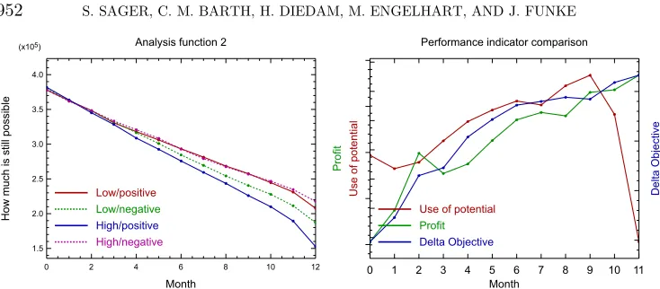
4.2. Impact of emotion regulation. In the study 174 data sets were used, every one from a different participant who had but one try. For 42 of thempositive feedback
was used in the sense that in every round, regardless of the decisions the participant took, a sum of 20000 money units (MUs) was added to the capital. For 42 participants
negative feedbackin the form of a reduction of 8000 MUs was implemented. These
mod-ifications are implemented in the model and readjusted in the a posteriori analysis, of course.
In a previous study [5] it was shown that participants who receive negative feedback perform better than those who receive positive feedback. In our new study we additionally considered the ability to regulate emotion. The psychological results of this study are explained in [4] in which details on the experimental setup can also be found. As a main result, an interaction between feedback and emotion regulation could be shown: participants with a high ability of emotion regulation perform better when they get negative feedback, while those with a low ability to regulate their emo-tions perform badly for negative and well for positive feedback. This is illustrated in Figure 4.2(left).
In a second study, films and music were used to induce happy, neutral, and sad effects. Additionally we measured emotion regulation. The study was based on data from 90 participants, 30 in each effect condition. Again, emotion regulation had a great impact on complex problem solving. A high ability to regulate emotion improved com-plex problem solving and reduced the number of mistakes.
FIG. 4.2. Left: Average values of theHow much is still possible–function over all participants with emotion regulation properties/feedback a) low/positive, b) low/negative, c) high/positive, d) high/negative. Partici-pants with a low ability of emotion regulation performed better with positive feedback; those with high ability of emotion regulation performed better with negative feedback. Right: Average values over all174participants for different indicator functions. The Use of potential–function ΔPk is given by (4.1). Profit indicates
ΔxCA
k ¼xCAkþ1−xCAk , Delta objective indicatesΔxOBk ¼xOBkþ1−xOBk . The trajectories have been rescaled for
5. Summary and outlook. We presented a challenging problem class of noncon-vex MINLPs. They originate from economic test scenarios that are used in the analysis of human complex problem solving. Starting fromGW-Basicsource code of the test scenario we developed a mathematical optimization model to optimize performance starting from prespecified initial values. This model needed to be reformulated in several ways to avoid nondifferentiabilities, division by zero, and unboundedness.
TheTailorshop test scenario was invented more than 25 years ago, without any
intention to set it up suited for mathematical optimization. Our study revealed several shortcomings of the model. This insight can be used for defining better test scenarios in the future. All characteristics such as nondifferentiabilities, random values, or un-bounded decision variables should be left out, as they do not really contribute to the difficulty of the scenario itself but mainly to the difficulty of solving the problem math-ematically to optimality.
We solved altogether 2088 optimization problems and discussed the role of integer variables and the nonconvexity by comparing different algorithms. The difficulties in doing so for a large number of medium-scale nonconvex MINLPs are challenging. We formulated and used a structure exploiting lower bound to exclude certain unwanted local maxima. The optimization results were used in two ways. First, to gain additional insight into individual performance by comparing it to the optimal solution which is often nonobvious. Second, to use the results in an automated way as a new analysis tool for process-dependent evaluation of the performance.
This novel methodology yields a valuable (and accessible [45]) analysis tool for psychologists to evaluate participants’performance. We discussed why there is no alter-native to the How much is still possible–function, especially when participants have more insight, e.g., by repetition of tests. Furthermore, we proposed to add artificial constraints to the optimization problem and use the Lagrange multipliers of these con-straints as an indication of what decisions contributed significantly to good or bad per-formance. By providing this mathematical technology to analyze participants’decisions in more detail, a whole set of interesting scenarios with a time- and decision-specific resolution can be included in future psychological investigations.
This paper provides a reference for researchers in complex problem solving. But we also hope for a stimulating effect on optimization. Future studies should concentrate on restarts for the MINLPs, on a comparison with active-set based solvers, problem-specific cuts, tight bounds also for nonlinear subexpressions, and on more efficient techniques to find global optima.
Appendix. A.
A.1. Details of the optimization model. We list several parameters and initial values that are of relevance for the optimization problem (2.1) in Tables A.1 and A.2. Figure A.1 shows an extract of the original source code.
A.2. Derivation of the optimization model. We discuss some properties of (2.1) in more detail.
The only clearly defined integer variable within theGW-Basiccode is the choice of the showroom where the shirts are being sold. There are only three choices: city center, city, and suburbs, which we identify with 2, 1, and 0, respectively. We define
f1ðuCS
k Þ≔
8 > > < > > :
1.2 if uCS
k ¼2
1.1 if uCS
k ¼1
1.0 if uCS
k ¼0
; f2ðuCS
k Þ≔
8 > > < > > :
2000 if uCS k ¼2; 1000 if uCS
k ¼1; 500 ifuCS
k ¼0.
TABLEA.1
Fixed initial valuesx0and parametersp. Note that some initial values are not needed, as they do not enter the right-hand-side functionGð·Þ. Note also that units are only implicitly given in the test scenario.
State[unit] xk x0¼
machines 50 [machines] xM50k 10
shirts stock [shirts] xSTk 80.7164
machines 100 [machines] xM100
k 0
vans [vans] xVAk 1
workers 50 [workers] xW50
k 8
material stock [shirts] xMSk 16.06787
workers 100 [workers] xW100k 0
machine capacity [shirts] xMCk 47.04
demand [shirts] xDEk 766.636
capital after interest [MU1] xCA
k 165774.66
Parameter[unit] p p¼
max. demand [shirts] pMD 900
interest rate [—] pIR 0.0025
max. machine capacity [shirts] pMM 50
debt rate [—] pDR 0.0066
max. satisfaction [—] pMS 1.7
1MU means money units.
TABLEA.2
Fixed, but time-dependent, parametersp. Note that onlypPRk has an implicitly given unit. The other para-meters are dimensionless.
k pPR
k [MU1] pDEk [—] pP50k [—] pP100k [—]
0 4.00000 0.616192 0.583334 0.178080
1 4.09497 0.269502 0.080131 0.365665
2 8.26718 0.692422 0.599074 0.725099
3 4.87143 0.844487 0.177331 0.207369
4 4.85305 0.697927 0.075705 0.092567
5 5.90983 0.253290 0.669259 0.318009
6 5.18731 0.805071 0.587936 0.056364
7 7.09909 0.457335 0.107187 0.543777
8 6.77216 0.889342 0.788597 0.157994
9 7.61718 0.371173 0.370508 0.746488
10 8.02385 0.029353 0.908646 0.204585
11 2.68115 0.362480 0.166743 0.303585
To be able to relax the feasible set ofuCSk , we write these functions as
f1ðuCS
k Þ≔1þu CS k
10 ; f2ðuCSk Þ≔500þ250uCSk þ250uCSk ·uCSk :
For optimization algorithms the existence of tight lower and upper bounds makes a huge difference in runtime. By a process of trial and error we found several bounds that were never violated by any optimal or participant control. We define the feasible setΩof the control variables as given by the conditions (2.18)–(2.24).
A.2.2. Reformulations. Although there are some shortcomings in the economic model and the mathematical representation including nondifferentiabilities and no tight bounds on the variables is everything but favorable for a fast and reliable solution, we had to postpone the formulation of test scenarios with better properties to future work since most of the data of the 174 participants had already been evaluated when the interdisciplinary cooperation started. Hence the main issue was to reformulate the op-timization problem to be able to solve it under the constraint to keep it compatible with the available data.
Concerning nondifferentiability we strived to formulate the problem as a smooth optimization problem to allow more solvers to be able to treat the problem instances, if possible without additional binary variables.
As a first example, consider the state progression equation for the machine capacity xMC
k . A direct translation of the code would read as
xMC kþ1¼min
pMM;0.9xMC
k þ0.017 u
MA k
xM50
kþ1þ10−8xMkþ1001
:
ðA:1Þ
What was intended here was to include a safeguard to avoid division by zero by using xM50
kþ1þxkMþ1001 þ10−8as the denominator, but theGW-Basicimplementation used for the
evaluation includes the erroneous first version. In our model we add10−8to the denomi-nator in (A.1) to avoid division by zero but get comparable values forxMCkþ1.
Intuitively the fact that we are dealing with a nonconvex model and that there are no bounds on the variables probably means that the problem is unbounded. Indeed, the analysis of optimization results confirmed that due to a combination of a modeling error and the unboundedness of the controls it is possible to drive the overall profit to infinity. In the equation that describes the overall demand
xDE kþ1¼aþ
min
uAD
k 5 ; pMD
þ100xVA kþ1
·b
there is an upper bound on the effect of the advertisementuADk by means of a min ex-pression but not on the impact of vansxVAk . In other words, by buying more and more vans you can create an arbitrarily high demand. Demand itself enters into the number of shirts sold
xSS
kþ1 ¼min
xST
k ;54
xDE
k
2 þ280
·2.7181−u SP2 k 4250
:
Therefore you can sell an arbitrarily high number of shirts, if only you buy enough vans. However, none of the participants detected this error in the model—this only happened in a related study where participants got several repetitions. We discussed several ways to remove this unboundedness from the problem, e.g., setting a lower bound on the ca-pital to avoid unrealistic infinite debts, possibly by fixing this lower bound to the lowest value over all data sets to keep things consistent. However, the effect of the vans was still too strong. Eventually we decided to fix the number of vans in the optimization problem to exactly that of the respective participant and to focus on the other decisions that need to be taken.
The two expressions
xSA kþ1¼min
pMS;1
2þ
uWA
k −850
550 þ uSC k 800 ;
ðA:2Þ
xDE kþ1¼min
uAD
k 5 ; pMD
ðA:3Þ
can be directly replaced by
xSA
kþ1¼12þu WA
k −850
550 þ uSC k 800; 1 2þ uWA
k −850
550 þ
uSC k
xDE kþ1¼u
AD k 5 ;
uAD k
5 ≤pMD: ðA:5Þ
We replace the remaining min–max expressions by introducing sPP
k ≈minðxPPkþ1; xMSk þuΔkMSÞ;
ðA:6Þ
sMC
k ≈min
pMM;0.9xMC
k þ0.017 u
MA k
xM50
kþ1þ10−8xkMþ1001 þ10−8
;
ðA:7Þ
sSS
k ≈min
xST
k þxAPkþ1;54
xDE
k
2 þ280
·2.7181− uSP2k
4250
;
ðA:8Þ
sM50
k ≈minðxWkþ501; xMkþ501Þ;
ðA:9Þ
sM100
k ≈minðxWkþ1001 ; xMkþ1001Þ;
ðA:10Þ
and adding the corresponding constraints (2.27)–(2.31).
A constraint that states that new machines may only be bought when the machine capacityxMCk has at least the value of 35, or in other form
0≤uΔM100
k ≤
0 if xMC k <35;
∞ if xMC
k ≥35
ðA:11Þ
would be a little bit more tricky to reformulate in a way that is suited for a derivative-based optimization algorithm. Fortunately, due to the model bug in (A.1),xMCk will often be at its upper boundpMMin optimal solutions. The model error whenever a participant should havexMCk <35seems thus acceptable. Thus we simply ignore constraint (A.11). Another issue is the interest rates, which have a constant value but a different one for positive or negative capital xBCkþ1. This nondifferentiability in the right-hand side could be smoothed out easily by defining an appropriate function piecewise with the constant valuepIRforxBCkþ1≥δ, the constant valuepDRforxBCkþ1 ≤ −δ, and a smoothing function for the interval½−δ;δ, e.g., based on an arcus tangens. However, to facilitate implementation, we chose to use only the positive interest rate pIR. Whenever the optimal solution does not require lending money (hence no xBCk <0 for any month k), obviously without loss of generality, this solution is also optimal for the case with the higher interest rate. This requires another postprocessing that we needed to automatize.
The absolute value that occurs in the right-hand side of the statexPPkþ1 can be ne-glected because of the lower bound of 850 for the wagesuWAk .
Acknowledgment. We thank Andreas Potschka for helpful comments and suggestions.
REFERENCES
[1] K. ABHISHEK, S. LEYFFER,ANDJ. T. LINDEROTH,Filmint: An outer-approximation-based solver for non-linear mixed integer programs, Preprint ANL/MCS-P1374-0906, Argonne National Laboratory, Mathematics and Computer Science Division, 2006.
[2] J. ALBERSMEYER ANDM. DIEHL,The lifted Newton method and its application in optimization, SIAM J.
[3] D. APPLEGATE, R. E. BIXBY, V. CHVÁTAL, W. COOK, D. ESPINOZA, M. GOYCOOLEA,ANDK. HELSGAUN, Certification of an optimal TSP tour through85,900cities, Oper. Res. Lett., 37 (2009), pp. 11–15. [4] C. M. BARTH,The Impact of Emotions on Complex Problem Solving Performance and Ways of Measuring
This Performance, PhD thesis, Ruprecht–Karls–Universität Heidelberg, 2010.
[5] C. M. BARTH AND J. FUNKE,Negative effective environments improve complex solving performance, Cognition and Emotion, 24 (2010), pp. 1259–1268.
[6] P. BELOTTI,Couenne: A User’s Manual, Technical report, Lehigh University, 2009; also available online from https://projects.coin-or.org/Couenne/browser/trunk/Couenne/doc/couenne-user-manual .pdf?format=raw.
[7] L. T. BIEGLER,An overview of simultaneous strategies for dynamic optimization, Chemical Engrg. and Processing, 46 (2007), pp. 1043–1053.
[8] T. BINDER, L. BLANK, H. G. BOCK, R. BULIRSCH, W. DAHMEN, M. DIEHL, T. KRONSEDER, W. MARQUARDT, J. P. SCHLÖDER,ANDO. V. STRYK,Introduction to model based optimization of chemical processes on moving horizons, in Online Optimization of Large Scale Systems: State of the Art, M. Grötschel, S. O. Krumke, and J. Rambau, eds., Springer, 2001, pp. 295–340.
[9] R. E. BIXBY, M. FENELON, Z. GU, E. ROTHBERG,ANDR. WUNDERLING,Mixed-integer programming: A pro-gress report, in The Sharpest Cut: The Impact of Manfred Padberg and His Work, SIAM, Philadelphia, 2004, pp. 309–325.
[10] P. BONAMI, L. T. BIEGLER, A. R. CONN, G. CORNUÉJOLS, I. E. GROSSMANN, C. D. LAIRD, J. LEE, A. LODI,
F. MARGOT, N. SAWAYA, ANDA. WÄCHTER,An algorithmic framework for convex mixed integer nonlinear programs, Discrete Optim., 5 (2009), pp. 186–204.
[11] P. BONAMI, M. KILINC,ANDJ. LINDEROTH,Algorithms and software for convex mixed integer nonlinear programs, IMA Volumes, to appear.
[12] B. BREHMER,Feedback delays in dynamic decision making, Complex Problem Solving: The European Perspective, Lawrence Erlbaum Associates, 1995, pp. 103–130.
[13] M. R. BUSSIECK,GAMS Performance World,http://www.gamsworld.org/performance. [14] GAMS Development Corporation, GAMS homepage.http://www.gams.com/.
[15] D. DANNER, D. HAGEMANN, A. SCHANKIN, M. HAGER,ANDJ. FUNKE,Beyond IQ. a latent state-trait analysis of general intelligence, dynamic decision making, and implicit learning, Intelligence (2011) (in press). [16] D. DÖRNER,On the difficulties people have in dealing with complexity, Simulation and Games, 11 (1980),
pp. 87–106.
[17] P. H. EWERT ANDJ. F. LAMBERT,PartII: The effect of verbal instructions upon the formation of a concept,
J. of General Psychology, 6 (1932), pp. 400–411.
[18] C. A. FLOUDAS, I. G. AKROTIRIANAKIS, S. CARATZOULAS, C. A. MEYER,ANDJ. KALLRATH,Global optimiza-tion in the21st century: Advances and challenges, Comput. Chem. Eng., 29 (2005), pp. 1185–1202. [19] R. FOURER, D. M. GAY,ANDB. W. KERNIGHAN,AMPL: A Modeling Language for Mathematical
Program-ming, Duxbury Press, 2002.
[20] P. A. Frensch and J. Funke,EDS., Complex Problem Solving: The European Perspective, Lawrence
Erlbaum Associates, 1995.
[21] J. FUNKE,Einige Bemerkungen zu Problemen der Problemlöseforschung oder: Ist Testintelligenz doch ein Prädiktor?, Diagnostica, 29 (1983), pp. 283–302.
[22] J. FUNKE,Using simulation to study complex problem solving: A review of studies in the FRG, Simulation and Games, 19 (1988), pp. 277–303.
[23] J. FUNKE,Problemlösendes Denken, Kohlhammer, 2003.
[24] J. FUNKE,Complex problem solving: A case for complex cognition?, Cognitive Processing, 11 (2010), pp. 133–142.
[25] J. FUNKE ANDP. A. FRENSCH, Complex problem solving: The European perspective–10years after, Learning to Solve Complex Scientific Problems, Lawrence Erlbaum Associates, 2007, pp. 25–47. [26] C. GONZALEZ,Learning to make decisions in dynamic environments: Effects of time constraints and
cog-nitive abilities, Human Factors, 46 (2004), pp. 449–460.
[27] C. GONZALEZ, P. VANYUKOV,ANDM. K. MARTIN,The use of microworlds to study dynamic decision making,
Computers in Human Behavior, 21 (2005), pp. 273–286.
[28] A. GRÖSSLER, F. H. MAIER,ANDP. M. MILLING,Enhancing learning capabilities by providing transparency in business simulators, Simulation & Gaming, 31 (2000), pp. 257–278.
[29] I. E. GROSSMANN,Review of nonlinear mixed-integer and disjunctive programming techniques, Optim.
Eng., 3 (2002), pp. 227–252.
[30] H. J. HÖRMANN ANDM. THOMAS,Zum Zusammenhang zwischen Intelligenz und komplexem Problemlösen,
[31] W. HUSSY,Komplexes Problemlösen—Eine Sackgasse?, Zeitschrift für Experimentelle und Angewandte
Psychologie, 32 (1985), pp. 55–74.
[32] W. HUSSY, Komplexes Problemlösen und Verarbeitungskapazität, Sprache & Kognition, 10 (1991),
pp. 208–220.
[33] M. KLEINMANN ANDB. STRAUSS,Validity and applications of computer simulated scenarios in personal assessment, International J. of Selection and Assessment, 6 (1998), pp. 97–106.
[34] R. H. KLUWE,Knowledge and performance in complex problem solving, The Cognitive Psychology of Knowledge, Elsevier Science Publishers, 1993, pp. 401–423.
[35] Z. H. KLUWE, C. MISIAK,ANDH. HAIDER, Systems and performance in intelligence tests, Intelligence: Reconceptualization and Measurement, Lawrence Erlbaum Associates, 1991, pp. 227–244. [36] S. KOLB, F. PETZING,ANDS. STUMPF,Komplexes Problemlösen: Bestimmung der Problemlösegüte von
Probanden mittels Verfahren des Operations Research—ein interdisziplinärer Ansatz, Sprache & Kognition, 11 (1992), pp. 115–128.
[37] B. MEYER ANDW. SCHOLL,Complex problem solving after unstructured discussion. Effects of information distribution and experience, Group Process and Intergroup Relations, 12 (2009), pp. 495–515. [38] J. A. NELDER ANDR. MEAD,A simplex method for function minimization, Computer Journal, 7 (1965),
pp. 308–313.
[39] M. OSMAN, Observation can be as effective as action in problem solving, Cognitive Science: A
Multidisciplinary Journal, 32 (2008), pp. 162–183.
[40] J. H. OTTO AND E.-D. LANTERMANN, Wahrgenommene Beeinflussbarkeit von negativen Emotionen, Stimmung und komplexes Problemlösen, Zeitschrift für Differentielle und Diagnostische Psychologie, 25 (2004), pp. 31–46.
[41] W. PUTZ-OSTERLOH,Über die Beziehung zwischen Testintelligenz und Problemlöseerfolg, Zeitschrift für Psychologie, 189 (1981), pp. 79–100.
[42] W. PUTZ-OSTERLOH, B. BOTT,ANDK. KÖSTER,Models of learning in problem solving–are they transferable to tutorial systems?, Computers in Human Behavior, 6 (1990), pp. 83–96.
[43] T. W. ROBBINS, E. J. ANDERSON, D. R. BARKER, A. C. BRADLEY, C. FEARNYHOUGH, R. HENSON, S. R. HUDSON,ANDA. BADDELEY, Working memory in chess, Mem. Cognit., 24 (1996), pp. 83–93. [44] S. SAGER,Reformulations and algorithms for the optimization of switching decisions in nonlinear optimal
control, J. of Process Control, 19 (2009), pp. 1238–1247.
[45] S. SAGER, H. DIEDAM,ANDM. ENGELHART,Tailorshop: Optimization Based Analysis and Data Generation Tool, TOBAGO web sitehttps://sourceforge.net/projects/tobago.
[46] S. STROHSCHNEIDER ANDD. GÜSS,The fate of the moros: A cross-cultural exploration of strategies in com-plex and dynamic decision making, International J. of Psychology, 34 (1999), pp. 235–252. [47] H.-M. SÜSS, K. OBERAUER, ANDM. KERSTING,Intellektuelle Fähigkeiten und die Steuerung komplexer
Systeme, Sprache & Kognition, 12 (1993), pp. 83–97.
[48] M. TAWARMALANI ANDN. SAHINIDIS,Convexification and Global Optimization in Continuous and Mixed-Integer Nonlinear Programming: Theory, Algorithms, Software, and Applications, Kluwer Academic Publishers, Dordrecht, The Netherlands, 2002.
[49] M. TAWARMALANI ANDN. V. SAHINIDIS,A polyhedral branch-and-cut approach to global optimization,
Math. Program., 103 (2005), pp. 225–249.
[50] A. WÄCHTER ANDL. T. BIEGLER,On the implementation of an interior-point filter line-search algorithm for large-scale nonlinear programming, Math. Program., 106 (2006), pp. 25–57.
[51] D. WAGENER,Personalauswahl und -Entwicklung mit komplexen Szenarios, Wirtschaftspsychologie, 3 (2001), pp. 69–76.
[52] D. WENKE ANDP. A. FRENSCH,Is success or failure at solving complex problems related to intellectual ability?, The Psychology of Problem Solving, Cambridge University Press, Cambridge, U.K., 2003, pp. 87–126.