603
Volume 64 72 Number 2, 2016
http://dx.doi.org/10.11118/actaun201664020603
THE EMPIRICAL IMPLICATIONS OF THE ZERO
LOWER BOUND ON THE INTEREST RATE:
THE CASE OF THE CZECH ECONOMY
Miroslav Hloušek
11 Faculty of Economics and Administration, Masaryk University, Lipová 41a, 602 00 Brno, Czech Republic
Abstract
HLOUŠEK MIROSLAV. 2016. The Empirical Implications of the Zero Lower Bound on the Interest Rate: The Case of the Czech Economy. Acta Universitatis Agriculturae et Silviculturae Mendelianae Brunensis,
64(2): 603–616.
This paper uses an estimated DSGE model of the Czech economy to study the macroeconomic implications of various shocks when the interest rate is constrained by the zero lower bound. The goal is to identify which shocks represent threats for the economy and how large the distortions are. The results show that four single shocks can take the economy to the zero lower bound, and that of the four, productivity shock in the tradable sector is the most dangerous. The consequences for the behaviour of macroeconomic variables are nontrivial and, quite naturally, increase with the size of the shock and the frequency of occurrence. If the economy is subject to all model specifi c shocks, there are distortions in terms of lower average values of output and consumption (by more than one percentage point) and higher infl ation volatility (by more than six percentage points). To reduce these costs, the central bank should give higher weight to infl ation and lower weight to the output gap in monetary policy rule.
Keywords: zero lower bound on interest rate, DSGE model, occasionally binding constraint, monetary policy
INTRODUCTION
Many developed economies have experienced near-zero interest rates in the last few years. This is illustrated in Fig. 1. The United States and European countries (including the Czech Republic) have joined Japan, which has had consistently low interest rates since the 1990s. The situation in these economies is similar: they are slowly recovering from the recession and there are defl ation pressures. This calls for expansionary economic policy to promote growth and increase prices. Monetary policy should respond by reducing interest rates, but this is not possible because the interest rates are near zero and cannot be negative.1 This situation is
called the liquidity trap or zero lower bound (ZLB) on interest rates. Naturally, it has consequences for the whole economy, which are worth exploring. The goal of this paper is to empirically assess the implications of the zero lower bound on the interest rate for macroeconomic variables in the Czech economy. Concretely, a DSGE model is estimated on Czech data by Bayesian techniques and a series of simulations is carried out. The types and sizes of disturbances that can push the interest rate to the zero lower bound are identifi ed, as are the consequences this has for macroeconomic variables. The results show that for the interest rate conditions that prevail in mid-2015, four shocks could take the economy to the zero lower bound with a
time impact. They are: productivity shock in the tradable sector, labour supply shock, monetary policy shock and productivity shock in the non-tradable sector. Of these, productivity shock in the tradable sector is the most “dangerous” and has nontrivial consequences for consumption, output and infl ation behaviour. When a series of single shocks (similar in magnitude and persistence to those the Czech economy has experienced recently) is simulated, some other shocks arise as signifi cant for the ZLB, but their impacts for macroeconomic variables are trivial. When a combination of all model specifi c shocks hits the economy, the output is lower by around 1.16 percentage points on average and its standard deviation increases by more than one percentage point. The impacts on consumption are even stronger. Quite surprisingly, average infl ation is unchanged, but its volatility increases by more than six and half percentage points. To diminish these distortions, monetary policy should be more aggressive, placing greater weight on infl ation, and should pursue strict infl ation targeting (no weight on output).
LITERATURE REVIEW
The empirical consequences of the ZLB environment have been studied e.g. by Coenen
et al. (2004), who ran a simulation of a small
structural model subject to stochastic shocks similar in magnitude to those experienced in the U.S. during the 1980s and 1990s. They found that the ZLB constraint causes negligible distortions to macroeconomic variables if the infl ation target is two percent. However, for infl ation targets between zero and one, the volatility of output increases signifi cantly and the volatility of infl ation increases as well, albeit to a smaller extent. Gust et al. (2013) focus on the empirical implications of the ZLB in the U.S. economy during the Great Recession.
They look at which shocks took the U.S. economy to the lower bound, and how much this constraint contributed to severity of the Great Recession. In a hypothetical situation in which monetary policy was not constrained, the GDP would have been one percent higher over the years 2009–2011. Ireland (2011) also argues that the U.S. economy would recover from the recession sooner and more quickly without this constraint on the interest rate.
Only a few papers have dealt with ZLB issues in relation to the Czech economy. Franta et al. (2014) discuss the use of exchange rate interventions as a solution for the situation of the zero lower bound on the interest rates. They confi rm the suitability of this alternative monetary policy tool in the Czech economic conditions. Malovaná (2015) examines the eff ects of various shocks under diff erent monetary policy regimes when the economy is at the ZLB. She fi nds that when the economy is at the ZLB, the volatility of the real and nominal variables is amplifi ed in reaction to domestic demand shock, foreign demand and fi nancial shocks and terms of trade shocks. When the central bank fi xes nominal exchange rate at ZLB, it helps to mitigate defl ationary pressures and to recover economic activity. Hloušek (2014) analyses a small open economy model estimated using Bayesian techniques on Czech data. The results show that the shocks likely to take the economy to the ZLB are domestic cost-push shock and foreign preference shock. The constraint on the interest rate has implications for consumption and output behaviour, but these are quantitatively small. This paper closely follows the strategy used in Hloušek (2014), but uses a larger model, extends the analysis for a broader combination of shocks, and discusses their impacts for monetary policy. Finally, Hloušek (2016) also deals with the impacts of the zero lower bound for the macroeconomy, but his research question is focused on infl ation target setting by the central bank.
1: Development of interest rates in selected economies
Model Economy
The model used in this paper is borrowed from Kolasa (2009). The model structure is described only verbally here, and the full model equations are to be found in the Appendix. It is a model of two open economies, which are treated identically, and diff er only by their size, which is determined by the calibrated parameter n. The domestic economy represents the Czech economy, and the foreign economy is the Euro area.
There are two types of fi rm in every economy: producers of tradable goods and producers of non-tradable goods. The production function is Cobb-Douglas using capital and labour. The capital accumulation is subject to adjustment cost. The output is divided into consumption and investment goods. The tradable consumption and investment goods are combined with imports to make composite goods, a proportion of which are exported. There is assumed price rigidity at three stages of the production process. The rigidity is modelled in Calvo (1983) style and results in three price Phillips curves (for home tradable goods, non-tradable goods and composite consumption goods). Households consume a bundle of tradable and non-tradable goods, and decide about labour supply and bond purchases. There is an assumption of habit formation in consumption. Households have diff erent labour skills, which gives them the power to infl uence wages. The wage setting is subject to rigidity, which is again modelled according to Calvo (1983).
The government collects lump-sum taxes to fi nance its expenditures and always has a balanced budget. The government expenditures consist of domestic non-tradable goods and are modelled as an AR(1) process. Monetary policy follows the Taylor rule with interest rate smoothing and attention to infl ation and the output gap.
The model consists of forty structural equations and its dynamic is driven by seven exogenous shocks in each economy. Six of them follow AR(1): these are productivity shocks in the tradable sector and the non-tradable sector, a labour supply shock, an investment effi ciency shock, a consumption preference shock and a government spending shock. Monetary policy shock is assumed iid.
DATA AND METHODS
The methodology of estimation closely follows Kolasa (2009). The model is estimated using data for fourteen variables – GDP, consumption, investment, infl ation, real wages, nominal interest rate and internal exchange rate2 each for both the domestic and foreign economies. These data series are chosen so that they correspond to model variables that could be observed; their number
equals to the number of shocks in the model for the sake of identifi cation purposes. The time series enter as the growth rates and are demeaned before estimation. Only the nominal interest rate and price infl ation are used without transformation and are also demeaned. The data are quarterly and are taken from the Eurostat database, covering the time period 2001:Q2–2014:Q1. The time span is determined by the availability of data for the calculation of the internal exchange rate.
The model parameters are estimated using Bayesian techniques. A posterior distribution of the parameters is obtained by the Random Walk Chain Metropolis-Hastings algorithm. This generates 2,000,000 draws in two chains with 1,000,000 replications each; 90% of the replications are discarded so as to avoid any infl uence from initial conditions. MCMC diagnostics are used to verify the convergence. All computations are carried out using the Dynare toolbox (Adjemian et al., 2000) in Matlab so ware.
The estimated model is then simulated using the
Occbin toolbox developed by Guerrieri and Iacoviello
(2015), who use a piecewise linear perturbation method that is able to solve dynamic models with an occasionally binding constraint. This method provides a very good approximation of a dynamic programming solution but is much easier to implement and is much faster even for models with many state variables. This algorithm captures nonlinearities that arise in models with two regimes – with and without a binding constraint. Therefore, it is suitable for studying the eff ects of attaining the zero lower bound on the nominal interest rate.
Calibration and Estimation Results
Thirteen structural parameters are calibrated according to the data of national accounts. Ten structural parameters, seven standard deviations of shocks and six autoregressive parameters are estimated for each economy. The domestic and foreign shocks are allowed to correlate and the correlation coeffi cient is also estimated. The priors of the estimated parameters are set according to Kolasa (2009) and Slanicay (2013).
The results of the estimation are reported in Tab. A.I and A.II in the Appendix. Here, we look at just a few of the most relevant estimated parameters. The parameters of monetary policy rule are as follows: the posterior mean of the interest rate smoothing parameter is = 0.85, the weight to infl ation is = 1.37, and the weight to output gap is y = 0.07. These estimates are quite comparable with the results of other empirical studies for the Czech economy. The persistence and volatility of the shocks are reported in Tab. A. II and are key to our analysis. The most persistent shock is domestic productivity shock in the tradable goods sector,
aH = 0.91, while the least persistent is domestic productivity shock in the non-tradable goods sector,
aN= 0.45. The most volatile shock is domestic labour supply shock, with standard deviation σl = 0.345, while the least volatile is domestic monetary policy shock, σm = 0.002. Generally, the shocks in the Czech economy are more volatile than the shocks in the Euro area. A very high correlation was found between the two economies for monetary policy shocks.
Results from Model Simulation
The shocks and their impact for model behaviour form the core of our analysis. First, impulse response functions are used to study the variables’ reactions in response to positive and negative values of the shocks and the diff erences in the behaviour of these variables when the interest rate is and is not constrained by zero value is evaluated. Second, the model is simulated to a series of the shocks. The subject of interest is how o en the interest rate is binding and what the average duration of the ZLB period is. As in the previous case, the reactions of the macroeconomic variables in terms of their average values and volatility are compared. This analysis is carried out for each shock and for a combination of all fourteen model shocks.
The initial condition for the nominal interest rate is rather important for the results. As we are interested in the current situation of the Czech economy and the future possible cost of the zero lower bound constraint, the initial nominal interest rate is set to 0.3 percent annually, which corresponds to the 3M PRIBOR in the second quarter of 2015.
Impulse Responses
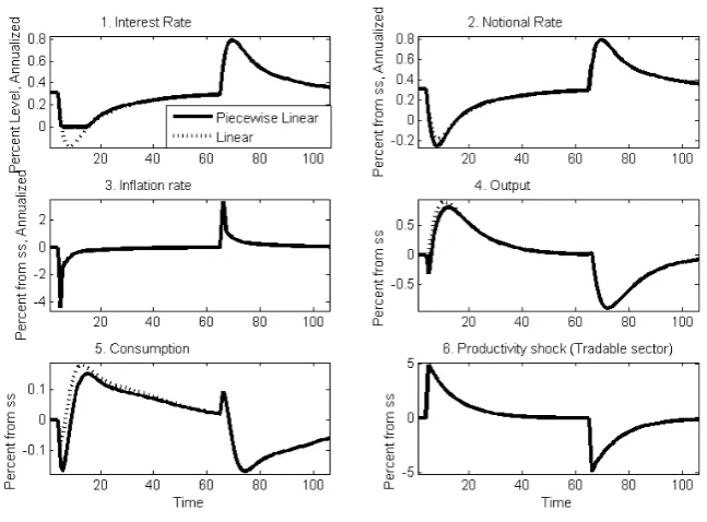
Fig. 2 shows the reaction of the model variables to a productivity shock in the tradable sector. The size of the shock is one standard deviation (posterior mean obtained from estimation). The y-axis shows the percentage deviation from the steady state, except for the fi rst subgraph, which is in percent level. The dotted line depicts the linear solution which corresponds to a situation in which the nominal interest rate is allowed to be negative. The solid line depicts the piecewise linear solution and corresponds to the zero lower bound case. Let us examine the linear solution fi rst. The economy is subject to positive productivity shock in period fi ve. This causes infl ation to decrease and output to increase. The central bank reacts to low infl ation by lowering the interest rate. Consumption initially drops because the high real interest rate makes consumption more expensive and forces people to postpone it for the future. A er this drop, consumption quickly rises above the steady state. In the piecewise linear solution, the central bank cannot decrease the nominal interest rate enough, because it hits the zero lower bound. The interest rate stays at zero value for ten periods and then moves in line with the linear solution. The constraint on the interest rate results in a larger initial drop in the infl ation rate (by around one percentage point). There is also a diff erence in the reactions of output and especially consumption. There is a stronger initial drop, and the trajectory in the ZLB case is lower for a longer time compared to the unconstrained version. The top right panel in Fig. 2 shows the impulse responses of the notional interest rate. The linear version is the same as the
2: Impulse responses to productivity shock in tradable sector (ZLB and noZLB case)
linear version for the nominal interest rate; the piecewise linear solution shows the interest rate’s behaviour if the central bank reacts to variables in the piecewise linear solution (ZLB case). As the infl ation rate decreases more, and because of the small initial drop in output, the central bank should respond with more expansionary monetary policy, i.e. by lowering the interest rate. A er sixty periods, the variables are back at steady state. Then a negative productivity shock hits the economy in period sixty fi ve. The reaction of the variables is a mirror image of the previous case, but now both solutions coincide, because the interest rate is not constrained.
This analysis is carried out for all fourteen shocks, and demonstrates that for four of them the interest rate is binding in at least one period. These are quoted in Tab. I together with the estimated standard deviation and number of periods when the interest rate was binding. Three sizes of shocks are assumed: one, two and three standard deviations.3 The pattern is as expected: the larger the shock, the longer the interest rate is binding. Of these four shocks, productivity shock in the tradable sector is the most distinct, even though its estimated standard deviation is only 5 percent. An example of such a shock is technological improvement in the engineering industry, which causes more goods to be produced with given resources. Even if this shock increases output, which may be considered a positive impulse during the recession, it decreases infl ation and thus forces the central bank to lower the interest rate, which becomes problematic at the ZLB.
Labour supply shock was estimated as the most volatile and is the second most “dangerous” shock in this analysis. Positive labour supply shock can be represented by a decrease in the weight of leisure in consumers’ utility, or some exogenous increase in labour force. This shock translates into higher output and consumption, and lower wages. The lower wages decrease marginal costs and thus infl ation, which is again a signal for the central bank to decrease the interest rate.
Monetary policy shock is the least volatile, but could take the economy to the ZLB for two periods. The reasoning is obvious: this shock directly infl uences the nominal interest rate. Productivity shock in the non-tradable sector only causes interest rate binding at larger values of this shock (two and three standard deviations).
As we have seen in Fig. 2, the zero lower bound can cause macroeconomic variables to behave diff erently in reaction to the shocks. First, we will quantify the diff erence at the peak (trough) of impulse responses. The upper panel of Fig. 3 shows the consumption reaction to diff erent sizes of productivity shock in tradable sector, up to three standard deviations, for both positive and negative values of the shocks. The size of the shock is given on the x-axis. The y-axis measures the percentage deviation of consumption from the steady state for both the ZLB and noZLB cases. The lower panel shows the diff erence between the two trajectories from the upper panel. For an average size shock (one standard deviation) the diff erence is negligible, however it increases non-linearly with the size of the shock. The drop in consumption is greater by 1.6 percentage points for a shock of three standard deviations.
The diff erences for other shocks and other macroeconomic variables (output and infl ation) are shown in Tab. II. The distortions correspond to the results from Tab. I. The productivity shock is the most “dangerous” and can cause signifi cant costs – lower consumption, output and infl ation.4 For average values of the shock, the costs are moderate. However, when a shock as large as three standard deviations hits the economy, output is reduced by four percentage points and infl ation by sixteen percentage points p.a. Such a situation is, of course, not very likely. Given the fact that innovations to the shocks are normally distributed, shocks bigger than three standard deviations are probable in just 0.3 % of cases. The costs caused by other shocks are much smaller, and correspond to the number of periods for which the economy stays at the ZLB.5 Labour
3 As the shocks are assumed to have a normal distribution, the one standard deviation covers 68.3% of all shocks, two standard deviations cover 95.4% and three standard deviations cover 99.7% of shocks that occur statistically in the economy.
4 Lower infl ation can be perceived as a benefi cial result, however if the infl ation is negative (defl ation) it brings costs
rather than benefi ts. 5 As indicated in Tab. I.
I: Binding interest rate for selected shocks
Posterior mean of std Interest rate is binding
1σ 2σ 3σ
Prod. shock – tradable sector 0.0491 10 17 20
Labour supply shock 0.3486 4 9 11
Monetary policy shock 0.0015 2 4 5
Prod. shock – non-tradable sector 0.0825 0 3 4
supply shock and monetary policy shock have non-negligible consequences for macroeconomic variables only when these shocks are large, and productivity shocks in the non-tradable sector have only trivial impacts.
Simulation in the Presence of Single Shocks
The situation we have just examined assumed that the shocks hit the economy only once and that their eff ects fade out with time. The next exercise assumes, on the contrary, that each shock occurs in a large number of periods. Most of the shocks follow the AR(1) process:
e.g. ϵg,t= gϵg,t−1 + g,t,
where the term “shock” is used for the variable ϵg,tand the term “innovation” for g,twhich has properties
g,t ~ N(0, g). Concretely, fi ve thousand random numbers from a normal distribution are generated and then multiplied by the estimated standard deviation of the particular shocks. These numbers correspond to the innovations. The shocks follow an autoregressive process with persistence parameters obtained from the estimation and the series of these innovations. Therefore, this construction should resemble the shocks that the Czech economy truly experienced during the estimated period. The
empirical distribution from this simulation in the presence of productivity shocks in the tradable sector is shown in Fig. 4. The solid line depicts the distribution for the ZLB case, while the dotted line indicates the case with a non-binding interest rate (no ZLB). It is clear that the distribution in the ZLB case is shi ed to the le for consumption and output, and to the right for infl ation. It corresponds to the results obtained from impulse responses. Statistical properties and other characteristics for all important shocks are shown in Tab. III. The second column shows the probability of the interest rate binding to the ZLB, the third column shows the average duration of its spell at the ZLB, and the fourth to seventh columns show the impact for macroeconomic variables in terms of median diff erences between the ZLB and noZLB cases.
As the shocks are quite persistent and several successive adverse innovations can occur, the probability that the economy reaches the ZLB and stays there is higher compared to impulse responses. The interest rate is binding for productivity shocks in the tradable sector and for labour supply shocks, in almost 40 percent of cases. These two shocks also exhibit non–trivial losses in terms of lower consumption and output. Productivity shocks in the tradable sector reduce the average consumption and output by 0.54 and 0.94 percentage points,
3: Response of consumption to a productivity shock in the tradable sector
Source: author’s calculations
II: Implications of the ZLB at impulse responses (diff erence ZLB – no ZLB in percentage points)
Impact on consumption Impact on output Impact on infl ation (p.a.)
1σ 2σ 3σ 1σ 2σ 3σ 1σ 2σ 3σ
Prod. shock – T sector –0.10 –0.76 –1.61 –0.27 –1.91 –4.04 –1.07 –7.72 –16.40
Labour supply shock –0.01 –0.15 –0.33 –0.02 –0.49 –1.13 –0.11 –1.95 –4.46
Monetary policy shock –0.02 –0.11 –0.22 –0.06 –0.32 –0.63 –0.22 –1.13 –2.26
Prod. shock – NT sector 0.00 0.00 –0.01 0.00 –0.03 –0.14 0.00 –0.09 –0.49
respectively, compared to the reduction with a non– binding interest rate. On the other hand, the impacts for infl ation are modest; its average value is higher by 0.72 p.p. (in annual terms). The reason is that the central bank is primarily concerned with targeting of infl ation and not output gap. Monetary policy shock also takes the economy to ZLB quite frequently, but its impacts for macroeconomic variables are trivial.
Furthermore, two new shocks play a role: investment effi ciency shocks in the domestic and foreign economies.6 However, compared to the shocks described above, their macroeconomic consequences are quite small and are comparable to the impacts of productivity shocks in the non-tradable sector. The longest average duration at the ZLB is around eight years, with a foreign investment effi ciency shock. This is quite surprising, because this shock does not take the interest rate to the ZLB so frequently. However, this outcome is robust to a number of simulations. Empirically, it can only be
compared to the situation of Japan, whose economy has been at the ZLB for such a long time. The average spell at the ZLB for the other shocks ranges from three quarters of a year to three years, which is a much more acceptable duration.
Before moving on to the last set of simulations, it is worth comparing these results with other empirical studies. Gust et al. (2013) also documented that productivity shocks played an important role for output decline during the Great Recession. Discount rate shocks had quite important consequences, but only for the behaviour of infl ation. Discount rate shocks correspond to preference shocks in our model, and they turned out to be unimportant in the analysis. This could be because the model used by Gust et al. contained only three types of shocks. Fernández-Villaverde et al. (2012) uses a small calibrated New Keynesian model with four shocks. The main source of distortions at the ZLB is ascribed to technology and discount
4: Empirical distribution for productivity shocks in the tradable sector
Source: author’s calculations
III: Simulation of reaction to single shocks
Binding IR (in %)
Avg spell (periods)
diff erence of median (p.p.) (ZLB – noZLB)
C Y π (p.a.)
Prod. shock – T sector 38.7 13.2 –0.54 –0.94 0.72
Labour supply shock 38.1 8.6 –0.16 –0.23 0.24
Monetary policy shock 34.2 3.0 –0.06 –0.06 0.12
Prod. shock – NT sector 16.1 3.0 –0.01 –0.02 0.04
Investment effi ciency shock 16.1 12.6 –0.01 –0.03 0.04
Fgn investment effi ciency shock 7.0 31.9 –0.03 –0.01 0
Source: author’s calculations
factor shocks, which both have similarly large impacts for macroeconomic variables. Hloušek (2014) found that, for the Czech economy, domestic cost-push shock, monetary policy shock and foreign preference shocks are the most signifi cant sources of welfare losses at ZLB. Contrary to his results, foreign shocks are not found to be important in taking the economy to the ZLB in our model. Malovaná (2015) identifi ed for the Czech economy that various demand shocks (both domestic and foreign) increase volatility of real and nominal variables at ZLB. Similarly to our results, positive domestic productivity shock weakens economic expansion at ZLB and thus leads to economic losses.
Simulation in the Presence of All Shocks
The results from the previous section can be seen as a lower bound, because the economy may be subject to a combination of several shocks. We will therefore explore the situation again, using a stochastic simulation, but this time the economy will be subject to all fourteen shocks. The results are shown in Tab. IV, which also shows the diff erences in volatilities between the ZLB and noZLB distributions. The fi rst row indicates that the interest rate is binding in almost half of the cases, and the average spell for which the economy stays at the ZLB is ten periods. The implications of the ZLB for macroeconomic variables are nontrivial. Consumption is lower by 1.72 percentage points on average, and output by 1.16 p.p. On the other hand, the average value of infl ation is almost unchanged. Regarding the volatilities of the variables, consumption is more volatile by one percentage point, output by half a percentage point and infl ation by as much as 6.52 p.p.
In sum, these results show that the empirical consequences of the ZLB are quite substantial, which raises the question as to whether anything can be done about it. To answer this question, we focus on the central bank’s behaviour, more concretely on diff erent settings of monetary policy
rule. The last two rows in Tab. IV show the results of the simulation for diff erent parameter values of the Taylor rule. First, the weight to output, parameter
y, is decreased from benchmark value y = 0.07 to 0.03, which is the lowest value found for the Czech economy in empirical papers, concretely in Ryšánek et al. (2012). The results of the simulation show that the ZLB occurs in fewer cases under these conditions. Quite surprisingly, the diff erence in the average values of output is unchanged, but there is improvement in consumption, whose average value in the ZLB case is lower by only 1.29 percentage points. Another improvement is in the volatility of consumption and output: the ZLB distribution for these two variables is now less volatile compared to the unrestricted version. Regarding infl ation, its average value is almost unchanged, but the diff erence in volatility has decreased compared to the benchmark. In other words, these results indicate that some form of strict infl ation targeting is benefi cial for the economy in an environment of low interest rates.
Next, we focus on increasing the weight to infl ation in monetary policy rule. It is increased from benchmark value = 1.37 to 1.94, which is the highest estimate for the Czech economy, again obtained from Ryšánek et al. (2012).7 The third row in Tab. IV shows the results of this simulation. The ZLB constraint binds in fewer cases compared to the benchmark, but only slightly. The other results are similar to the results with lower weight to output: a smaller diff erence in average values of consumption and almost no change for output and infl ation. Consumption is less volatile in the ZLB case by one percentage point and output is also somewhat less volatile. Infl ation is more volatile in the ZLB case, but there is improvement against the benchmark. The message of this experiment is that monetary policy that behaves more aggressively (higher weight to infl ation) lowers the distortions connected with the zero lower bound.
IV: Diff erences between descriptive statistics ZLB – noZLB
Binding IR Avg spell Diff erence of median (p.p.) Diff erence of std (p.p.)
C Y π (p.a.) C Y π(p.a.)
Benchmark MR 48.5 10.0 –1.72 –1.16 0.01 1.05 0.56 6.52
y = 0.03 44.1 8.3 –1.29 –1.16 –0.03 –0.51 –0.14 3.69
π = 1.94 47.0 9.2 –1.24 –1.14 0.00 –1.00 –0.17 3.08
Source: author’s calculations
7 The range of estimates for the Taylor rule parameters in the literature is quite wide. The infl ation parameter varies from
1.16 (Tonner et al., 2011) to 1.94 (Ryšánek et al., 2012) and the output gap parameter ranges from 0.03 (Ryšánek et al.,
CONCLUSION
This paper has explored the empirical consequences of attaining the zero lower bound on the interest rate in the Czech economy, using an estimated DSGE model. Of the fourteen model specifi c shocks, four shocks turned out to be important in determining the behaviour of the interest rate near the ZLB. They are: productivity shock in the tradable sector, labour supply shock, monetary policy shock and productivity shock in the non-tradable sector. The most signifi cant is the fi rst – productivity shock in the tradable sector, which means that more output can be produced with given inputs. In the case of the Czech economy, this can be represented e.g. by technological improvements in the engineering industry.
Individual shocks produce quite small welfare losses at one time impact. The costs become important only for shocks of very high magnitude (two or three standard deviations) or when shocks occur more frequently. E.g. if the economy is subject to a series of productivity shocks in the tradable sector, output could be lower by almost one percentage point and consumption by half a percentage point on average. If the economy is subject to a series of all fourteen shocks, the losses connected with the ZLB are even higher: average output is lower by 1.7 percentage points and consumption by 1.2 percentage points. Although the average value of infl ation is almost unchanged, its volatility (measured by standard deviation) increases by 6.5 percentage points annually in this situation.
In summary, this analysis has shown that the costs connected with the zero lower bound are quite substantial. The recommendation for monetary policy is therefore to pursue more aggressive behaviour and strict infl ation targeting (i.e. giving higher weight to infl ation and lower weight to output). There can be also room for unconventional policies, such as exchange rate interventions that can eliminate cost connected with zero lower bound. Exploration of their possible impacts on the economy is le for further research.
Acknowledgement
This paper is supported by specifi c research project No. MUNI/A/1049/2015 at Masaryk University and by research project of the Czech Science Foundation No. GA16-11223S.
REFERENCES
BRÁZDIK, F. 2011. An Announced Regime Switch: Optimal Policy for the Transition Period. Czech Journal of Economics and Finance, 61(5): 411–431. CALVO, G. 1983. Staggered prices in a
utility-maximizing framework. Journal of Monetary Economics, 12: 383–398.
COENEN, G., ORPHANIDES, A. and WIELAND, V. 2004. Price Stability and Monetary Policy Eff ectiveness when Nominal Interest Rates are Bounded at Zero. The B.E. Journal of Macroeconomics, 4(1): 1–25.
FRANTA, M., HOLUB, T., KRÁL, P., KUBICOVÁ, I., ŠMÍDKOVÁ, K. and VAŠÍČEK, B. 2014. Měnový kurz jako nástroj při nulových úrokových sazbách: případ ČR. In: Research and Policy Notes3. Czech National Bank.
GUERRIERI, L. and IACOVIELLO, M. 2015. Occbin: A Toolkit to Solve Models with Occasionally Binding Constraints Easily. Journal of Monetary Economics, 70: 22–38.
GUST, C., LOPEZ–SALIDO, D. and SMITH, M. E. 2012. The empirical implications of the interest– rate lower bound. Finance and Economics Discussion
Series, 2012–83. Board of Governors of the Federal
Reserve System (U.S.).
HLOUŠEK, M. 2014. Zero lower bound on interest rate: application of DSGE model on Czech economy. In: Proceedings of 32nd International
Conference Mathematical Methods in Economics.
Olomouc: Palacký University, 293–298.
HLOUŠEK, M. 2016. Infl ation Target and its Impact on Macroeconomy in the Zero Lower Bound Environment: the case of the Czech economy.
Review of Economic Perspectives, 16(1): 3–16.
IRELAND, P. N. 2011. A new Keynesian perspective on the great recession. Journal of Money, Credit, and Banking, 43: 31–54.
KOLASA, M. 2009. Structural heterogeneity or asymmetric shocks? Poland and the euro area through the lens of a two–country DSGE model.
Economic Modelling, 26(6): 1245–1269.
MALOVANÁ, S. 2015. Foreign Exchange Interventions at the Zero Lower Bound in the Czech Economy: A DSGE Approach. In: IES
Working Paper, 13/2015. Prague: IES FSV, Charles
University.
POLANSKÝ, J., TONNER, J. and VAŠÍČEK, O. 2011. Parameter Dri ing in a DSGE Model Estimated on Czech Data. Czech Journal of Economics and Finance, 61(5): 510–524.
RYŠÁNEK, J., TONNER, J., TVRZ, S. and VAŠÍČEK, O. 2012. Monetary policy implications of fi nancial frictions in the Czech Republic. Czech Journal of Economics and Finance, 62(5): 413–429
Appendix
This Appendix briefl y describes the structure of the domestic economy. The foreign economy has an identical structure. Parameters with an asterisk relate to the foreign economy. For further details about the model and log-linearized version, see Kolasa (2009).
Households
Households in a domestic economy are homogenous and maximize the expected utility function
, 1 , 1
=0
( ) = ( ( ) ) ( )
1 1
d t k l t k
k
t t t k t k t k
k
U j E C j H L j
,where Et denotes expectations in the period t,
is a discount factor, is an inverse elasticity of intertemporal substitution in consumption,
Ht = hCt−1 is an external habit taken by the household as exogenous, h isa parameter of habit formation, Ctis a composite consumption index (to be defi ned later),
is an inverse Frisch elasticity of labor supply, d,t is a preference shock in the period t, which infl uences intertemporal decisions about consumption and
l,t is a labor supply shock in the period t.
Households maximize the utility function subject to a budget constraint
PC,tCt(j) + PI,tIt(j) + Et{t,t+1Bt+1(j)} = Bt(j) + Wt(j)Lt(j) + + RK,tKt(j) + H,t(j) + N,t(j) + Tt(j), for t = 0, 1, 2, …, where PC,tdenotes the price of the consumption Ct, PI,t
isthe price of investment goods It, Bt+1 is the nominal payoff in period t + 1 of the portfolio held at the end of period t, Wt is the nominal wage, RK,t denotes income of households achieved from renting capital
Kt, H,t and N,tare dividends from tradable and non-tradable goods producers and Ttdenotes lump sum government transfers net of lump sum taxes. t,t+1 is the stochastic discount factor for nominal payoff s, such that Ett,t+1 = Rt−1, where Rtis the gross return on a riskless one-period bond.
Consumption index Ctconsists of fi nal tradable goods index CT,t and non-tradable goods index CN,t which are aggregated according to
1 , , 1 = (1 ) c c
T t N t
t c c
c c C C C ,
where c denotes the share of fi nal tradable goods in the consumption basket of households. It is assumed that consumption of a fi nal tradable good requires units of distribution services YD,t, which implies
CT,t = min{CR,t; −1Y
D,t}.
The consumption index of raw tradable goods is defi ned as
1 , , , = (1 )1
H t F t R t C C C ,
where denotes share of domestic goods in the domestic basket of tradable goods, CH,t is an index of home-made tradable goods and CF,t is an index of foreign-made tradable goods, both consumed in the domestic economy and defi ned as
1 1 1
, 0 1 = ( ) H H H n H H
H t t H H
C C z dz
n
,1 1 1
1 , 1 = ( ) 1 F F F F F
F t n t F F
C C z dz
n
,where H (F) is an elasticity of substitution between domestic (foreign) tradable goods, consumed in the domestic economy. Analogously, the consumption index of non-tradable goods is defi ned as
1 1 1
, 0 1 = ( ) N N N n N N
N t t N N
C C z dz
n
where N is an elasticity of substitution between domestic non-tradable goods.
Households use part of their income to accumulate capital Kt which is assumed to be homogenous and is rented to fi rms. Capital is accumulated according to the formula
1 ,
1
=(1 ) 1 t
t t i t t
t
I
K K S I
I ,
where is a depreciation rate of capital and Itdenotes investment in the period t. Capital accumulation is subject to investment specifi c technology shock i,t
and adjustment costs represented by function S(·). This function satisfi es following properties
S(1) = S(1) = 0 and S(·) = S>.
Homogenous investment goods are produced in the same way as fi nal consumption goods, which implies the following defi nitions
1 , , 1 = (1 ) i i
R t N t
t i i
i i I I I , 1 , ,
, = 1
(1 )
H t F t R t I I I .
diff er, i.e. parameters c and i can be diff erent, and that the composition of tradable baskets is identical, i.e. parameter is the same for both tradable consumption goods and tradable investment goods in the given economy.
Each household is specialized in a diff erent type of labour Lt(j), which it supplies in a monopolistically competitive labour market. All supplied labour types are aggregated into homogenous labour input
Lt according to the formula
1 1 1
0 1 = ( ) W W W n W W t t
L L j dj
n
,where W is the elasticity of substitution between diff erent labour types. A corresponding aggregate wage index is then defi ned as
1 1 1 0
1
= n ( ) W W
t t
W W j dj
n
,where Wt(j) denotes the wage of household j.
The setting of wages assumes Calvo (1983) mechanism. According to this set-up, every period only 1 − W portion of households (randomly chosen) can reset their wages optimally, while the remaining portion of households W leave their wages unchanged.
Firms
There is a continuum of homogenous, monopolistic competitive fi rms in the tradable and non-tradable sectors of the domestic economy. The production function of fi rms is assumed to be Cobb-Douglas function with constant returns to scale with respect to capital and labour
Yt(zN) = aN,tLt(zN)1−Kt(zN),
Yt(zH) = aH,tLt(zH)1−Kt(zH),
where is the elasticity of output with respect to capital (common to both sectors, but potentially diff erent in individual countries), and aH,t (aN,t) is a productivity shock in the tradable (non-tradable) sector.
Firms set their prices in order to maximize their profi ts. It is assumed that fi rms face Calvo (1983) pricing restriction. According to this restriction, every period only 1 − portion of fi rms (randomly chosen) have the opportunity to reset their prices optimally, while portion of fi rms leave their prices unchanged.
It is assumed that prices are set in the producer’s currency and that the international law of one price holds for intermediate tradable goods. Thus, prices
of domestic goods sold in the foreign economy and prices of foreign goods sold in the domestic economy are given by
Pt*(zH) = ERt−1P
t(zH), Pt(zF) = ERtPt*(zF), where ERt is the nominal exchange rate expressed as units of domestic currency per one unit of foreign currency.
International Risk Sharing
The assumption of complete fi nancial markets implies that expected nominal returns on domestic and foreign bonds must be the same, which implies the following condition
* * * * * , 1 1 , ( ) = ( )
d t t t
t
t t
d t
C h C Q C hC ,
where is a constant depending on initial conditions and Qt is a real exchange rate defi ned as
* ,
,
= t C t
t C t
ER P Q
P .
The real exchange rate can deviate from purchasing power parity because of changes in the relative prices of tradable and non-tradable goods, changes in relative distribution costs and changes in terms of trade, as long as there is a diff erence between household preferences among countries, i.e. 1 − *.
* *1 * * * 1 1 1 = 1 c t t
t t c
t t D X Q S D X ,
where St are the terms of trade defi ned as domestic import prices relative to domestic export prices8
* ,
,
= t F t
t H t ER P S
P .
Xt and Xt* are internal exchange rates defi ned as prices of non-tradable goods relative to prices of tradable goods
,
,
= N t t T t P X P , * , * * ,
= N t t
T t
P X
P
and Dt and Dt* are relative distribution costs, defi ned as prices of non-tradable goods relative to prices of raw tradable goods
,
,
= N t t R t P D P , * , * * ,
= N t t
R t P D
P .
Monetary and Fiscal Authorities
The behaviour of the central bank is described by a variant of the Taylor rule
1
, 1 1
1 ,
,
=
(1 )
y C t t
t t t m t
C t
P Y
R R E
Y P
,
where is a parameter of interest rate smoothing, Yt is a total output in the economy, Ytdenotes a steady state level of this output, is a steady state level of infl ation, y is an elasticity of the interest rate to the output, is an elasticity of the interest rate to infl ation and m,t is a monetary policy shock.
Fiscal policy is modeled in a simple way. Government expenditures and transfers to households are fully fi nanced by lump-sum taxes so that the state budget is balanced every period. Government expenditures consist only of non-tradable domestic goods and are modeled as a stochastic AR(1) process g,t. Given the assumptions about households, Ricardian equivalence holds in this model.
Market Clearing Conditions
The model is closed by the market clearing conditions. Goods market clearing requires that the output of each fi rm producing non-tradable goods is either consumed by households in the domestic economy, spent on investment, used for distribution services or purchased by the government. Similarly, the output of fi rms producing tradable goods is either consumed or invested in the domestic or foreign economy. Formally
YN,t = CN,t + IN,t + YD,t + Gt,
YH,t = CH,t + CH,t* + IH,t + I*H,t.
The total output in the economy is given by the sum of output in tradable and non-tradable sectors
Yt = YN,t + YH,t.
Finally, market clearing conditions for factor markets requires
0 0
= n ( ) n ( )
t t N N t H H
L
L z dz
L z dz ,0 0
= n ( ) n ( )
t t N N t H H
K
K z dz
K z dz .Exogenous Shocks
The business cycle behaviour of the model is driven by seven structural shocks in each economy: • productivity shocks in the tradable sector
(aH,t and *aF,t),
• productivity shocks in the non-tradable sector (aN,t and *aN,t),
• labour supply shocks (l,t and *l,t),
• investment effi ciency shocks (i,t and *i,t), consumption preference shocks (d,t and *d,t), • government spending shocks (g,t and *g,t) and • monetary policy shocks (m,t and *m,t).
A.I: Estimated parameters
Parameter Prior distribution Posterior distribution
Density Mean S.D. Mean 2.5% 97.5%
Habit formation
h beta 0.7 0.1 0.65 0.50 0.81
h* beta 0.7 0.1 0.73 0.60 0.86
Elasticity of intertemporal subst.
σ gamma 1 0.7 1.28 0.50 2.01
σ* gamma 1 0.7 2.52 1.24 3.76
Frisch elasticity of labour supply
gamma 1 0.7 0.37 0.01 0.78
* gamma 1 0.7 0.97 0.23 1.71
Investment adjustment cost
S norm 4 1.5 3.40 1.25 5.51
S* norm 4 1.5 4.73 2.69 6.59
Calvo parameters
H beta 0.7 0.05 0.75 0.69 0.81
*F beta 0.7 0.05 0.73 0.67 0.78
N beta 0.7 0.05 0.77 0.72 0.82
*N beta 0.7 0.05 0.63 0.57 0.69
W beta 0.7 0.05 0.73 0.65 0.80
W* beta 0.7 0.05 0.78 0.73 0.84
Monetary policy rule
beta 0.7 0.15 0.85 0.82 0.88
* beta 0.7 0.15 0.84 0.81 0.88
y gamma 0.25 0.1 0.07 0.05 0.09
*y gamma 0.25 0.1 0.13 0.07 0.18
π gamma 1.3 0.15 1.37 1.18 1.55
Contact information Miroslav Hloušek: hlousek@econ.muni.cz
A.II: Estimated shocks
Prior distribution Posterior distribution
Param. Density Mean S.D. Mean 2.5 % 97.5 %
Volatility
σaH invg 0.01 Inf 0.049 0.032 0.065
σ*aF invg 0.01 Inf 0.023 0.014 0.033
σaN invg 0.01 Inf 0.083 0.044 0.119
σ*aN invg 0.01 Inf 0.022 0.014 0.029
σd invg 0.01 Inf 0.038 0.015 0.060
σ*d invg 0.01 Inf 0.040 0.018 0.061
σl invg 0.01 Inf 0.349 0.085 0.653
σ*l invg 0.01 Inf 0.168 0.044 0.298
σg invg 0.01 Inf 0.032 0.027 0.037
σ*g invg 0.01 Inf 0.013 0.011 0.015
σi invg 0.01 Inf 0.073 0.026 0.116
σi* invg 0.01 Inf 0.033 0.020 0.044
σm invg 0.01 Inf 0.002 0.001 0.002
σ*m invg 0.01 Inf 0.002 0.002 0.002
Persistence of shocks
aH beta 0.7 0.1 0.91 0.82 0.93
*aF beta 0.7 0.1 0.63 0.62 0.96
aN beta 0.7 0.1 0.45 0.89 0.97
*aN beta 0.7 0.1 0.57 0.91 0.98
d beta 0.7 0.1 0.77 0.63 0.88
*d beta 0.7 0.1 0.73 0.63 0.86
l beta 0.7 0.1 0.45 0.28 0.67
*l beta 0.7 0.1 0.49 0.56 0.88
g beta 0.7 0.1 0.78 0.69 0.85
*g beta 0.7 0.1 0.81 0.73 0.89
i beta 0.7 0.1 0.66 0.48 0.82
*i beta 0.7 0.1 0.74 0.68 0.88
Correlation of shocks
corraH,a*
F norm 0 0.4 −0.02 −0.23 0.18
corraN,a*
N norm 0 0.4 0.24 0.05 0.44
corrd,d* norm 0 0.4 0.23 0.02 0.45
corrl,l* norm 0 0.4 0.12 −0.08 0.33
corrg,g* norm 0 0.4 0.12 −0.07 0.33
corri,i* norm 0 0.4 0.18 −0.01 0.39