Analysis of fibre-loop optical buffers
with a void-avoiding schedule
Wouter Rogiest
Ghent University, Dep. TELIN
St-Pietersnieuwstraat 41
9000 Gent, Belgium
[email protected]
Jan-Pieter Dorsman
Eindhoven University of
Technology
Centrum Wiskunde &
Informatica
[email protected]
Dieter Fiems
Ghent University, Dep. TELIN
St-Pietersnieuwstraat 41
9000 Gent, Belgium
dieter.fi[email protected]
ABSTRACT
In optical packet/burst switching, fibre-loop optical buffers pro-vide a compact and effective means of contention resolution. In case of fixed packet length, the involved loop length is typically chosen matched (equal to the packet length), and the loops are ar-ranged in parallel, constituting a single-stage buffer. In this contri-bution, we investigate the performance of such a buffer in an asyn-chronous network setting, assuming batch-Poisson arrivals and as-suming a so-called void-avoiding schedule. We show that by time-discretisation, the fibre-loop dynamics can be captured by a partic-ular type of exhaustive polling model. We obtain performance mea-sures such as the moments of the optical queue content and packet delay for the discretised model as well as for the asynchronous op-tical buffer. We illustrate our approach by various numerical exam-ples.
1.
INTRODUCTION
The major growth of personalised video streaming services and the paradigm shift toward big data all add to the bandwidth require-ments of Internet users, urging network providers to provision them with more capacity. While the current backbone network offers ca-pacities of over 10 Tbit/s per fibre, this capacity is only available for transmission from node to node. Current end-to-end communi-cation suffers capacity loss from inflexible switching in intermedi-ary nodes, urging for a more flexible approach to optical switching. Addressing this need, both optical burst switching (OBS) and opti-cal packet switching (OPS) provide alternatives, but require con-tention resolution in intermediate nodes, which can be done by means of buffering.
A feasible implementation of optical buffering is with pieces of fi-bre, employed either in a feed-forward set-up (where every line is traversed only once) [21] or, more compactly, as fibre loops. Many researchers (listed in [4]) have worked on implementations similar to the one proposed in [11]; recently, also a second type of imple-mentation with dual-loop optical buffers (DLOB) gained attention [13, 6, 22, 24]. Both types can accommodate for a single packet and are arranged in parallel in the design of loop optical buffers.
In this contribution, we provide a performance evaluation of a loop optical buffer with asynchronous operation, accommodating pack-ets with fixed lengthS. We assume a single loop length for all fibre loops, with actual delays amounting to multiples of this length. We assume that this length is matched to the packet length, i.e., the loop length isS.
The buffer is assumed located at the outgoing port of an optical switch, associated with a single wavelength outgoing fibre chan-nel. The buffer resolves contention between packets that request for transmission over the outgoing channel during overlapping time windows. Due to the nature of the delay medium, packets are de-layed somewhat more than strictly needed, receiving a delay that is realizable. Indeed, as packets recirculate within a fibre loop, re-alizable delays are within a given set{i·S}, withi=0,1,2.... Consequently, small timegapsorvoidsoccur in between packets transmitted on the outgoing channel, which are undesired in the sense that they reduce resource utilization of the channel’s capac-ity.
The functioning of a fibre-loop optical buffer is characterised by the reservation scheme, on the one hand, and the actual scheduling discipline, on the other hand. As proposed in [19], two reservation schemes can be identified.
1. Pre-reservation: packets may reserve the outgoing channel upon arrival, before entering the buffer. All contention is thus resolved at the input, by deciding on the exact delay before the packet enters one of the loops.
2. Post-reservation: packets do not reserve the outgoing chan-nel upon arrival, but only upon leaving their respective fibre loop. All contention is thus resolved at the output, by let-ting packets freely enter into the buffer, only deciding later on when a given packet exits its loop.
As can be intuitively understood, there is no benefit in reserving the outgoing channel earlier in time, since this prohibits rescheduling of packets present in the buffer as new packets arrive. This is firmed in [19], where the specific case of a single fibre loop is con-sidered. Essentially, post-reservation outperforms pre-reservation in terms of overall buffer performance, as it provides for better re-source utilization of the outgoing channel, with relatively smaller voids between successive outgoing packets. While post-reservation is thus the scheme with superior performance, preservation is the only option if no recirculation is possible in the given hardware, as in feed-forward optical buffers, analysed in e.g. [17], and in the often-cited [5].
3HUPLVVLRQWRPDNHGLJLWDORUKDUGFRSLHVRIDOORUSDUWRIWKLVZRUNIRU SHUVRQDORUFODVVURRPXVHLVJUDQWHGZLWKRXWIHHSURYLGHGWKDWFRSLHV DUHQRWPDGHRUGLVWULEXWHGIRUSURILWRUFRPPHUFLDODGYDQWDJHDQGWKDW FRSLHVEHDUWKLVQRWLFHDQGWKHIXOOFLWDWLRQRQWKHILUVWSDJH7RFRS\ RWKHUZLVHWRUHSXEOLVKWRSRVWRQVHUYHUVRUWRUHGLVWULEXWHWROLVWV UHTXLUHVSULRUVSHFLILFSHUPLVVLRQDQGRUDIHH
9$/8(722/6'HFHPEHU%UDWLVODYD6ORYDNLD &RS\ULJKWk,&67
'2,LFVWYDOXHWRROV
In terms of actual scheduling of packets, a broad variety of schedul-ing disciplines can be devised, operatschedul-ing either under a pre- or a post-reservation scheme. Key pre-reservation schemes for a single-wavelength buffer are
1. First-Come First-Served (FCFS): scheduling is done upon ar-rival. Packets are delayed for the smallest multiple of the loop durationSlarger than the time needed for all previ-ously arrived packets to have left the buffer, the so-called scheduling horizon. This approach corresponds to the pre-reservation scenario considered in [19], as well as to horizon scheduling (with pre-reservation required by the hardware) in [17].
2. Void-Filling: scheduling is done FCFS, unless a void in the existing provisional schedule allows for packets to be sched-uled in between, leading to better performance than FCFS. 3. Void-Creating: void-filling scheduling is modified by
selec-tively creating larger voids than strictly needed, only when these are likely to be filled later on [23], allowing for perfor-mance gain over void-filling.
Although for a different setting (without recirculation), [17] pro-vides results that are valid for the current setting if we enforce FCFS, which is a pre-reservation scheme.
For a post-reservation scheme, the scheduler is not forced to sched-ule packets upon arrival, allowing for more flexibility in terms of scheduling discipline. In this paper, we propose a scheduling dis-cipline called Void-Avoiding Schedule (VAS), which is quite in-tuitive, always trying to minimize voids on the outgoing channel, as explained below. VAS can be seen as a generalization of the scheduling discipline proposed in [19], where the same strategy is applied to a simpler setting of a single fibre loop. To the best of the authors’ knowledge, we are the first to study the case of post-reservation with a number of loops larger than one, which proves useful, as illustrated by the performance results, with significant deviation from the case of a single loop.
Somewhat surprisingly, the present study also relates to exhaustive polling models. Such models consist of a number of queues that are served by a single server. The server typically visits the queues in a cyclic manner in order to provide service at each of the queues. When the server has emptied a queue, it sets up for a visit to the next queue, which usually requires a positive and possible random switch-over time. The study of polling models originates from the late 1950s, when the papers of Mack et al. [14, 15] concerning a patrolling repairman model appeared. In a broader sense, polling models can be applied when several types of customers compete for access to a common resource which is available to only a single type of user at a time. Therefore, they find their origin in many present-day real-life applications, such as manufacturing environ-ments and traffic systems. The polling model particularly received a lot of interest during the 1980s, when it turned out to be a suit-able model for many computer-communication applications and protocols. This led to many seminal results, such as the pseudo-conservation law [3] and the connection with multi-type branch-ing processes [16] or semi-linear processes [1]. For an extensive overview of the literature on polling systems and an overview of their applications, we refer to surveys such as [2, 12, 20]. As a polling system, the continuous-time system considered in this
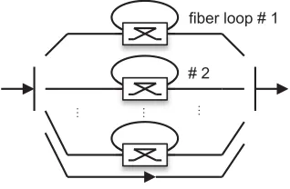
fiber loop # 1
… …
# 2
…
…
Figure 1: Parallelly-arranged loop optical buffer
paper strongly resembles yet differs from polling on a circle, as studied in [8, 10, 9, 18, 7]. In such a system, customers arrive at a circle according to a Poisson process, with position on the cir-cle determined as an independent and identically distributed (i.i.d.) random variable (uniform in [8, 9, 18], general i.i.d. in [10]), and wait for a single server who travels on the circle. Whenever the server encounters a customer, he stops and serves this customer, with i.i.d. service time. Compared to the fibre-loop model assumed here, a parallel can indeed be drawn, as the arrival process in the fibre-loop model is also Poisson, and the service time distribution is deterministic and thus also i.i.d. Further, due to the match of the loop length and the service time, one may indeed imagine a server moving around on a circle, travelling over the circle at constant pace in one direction, to finish the service at the exact same posi-tion where it started. Nevertheless, the two systems differ funda-mentally in two aspects. First, in a fibre-loop model, the customers do not enter the loop at i.i.d. locations, but the arrival process also moves around on the circle. Secondly, in a fibre-loop model, the server is allowed to make jumps whenever the system turns idle, as customers arriving in an idle system receive service immediately, rather than having to wait for the server to move toward them. In terms of greediness, as defined in [18], the server is non-greedy during busy cycles, but is somehow greedy at the start of the busy cycle. Due to these differences, the current model calls for an anal-ysis in its own right.
The remainder of this paper is organised as follows. The next sec-tion introduces the performance model of the fibre-loop buffer, with an infinite number of loops, and allow for an infinite number of recirculations. We show that by discretising time, the fibre-loop buffer can be exactly modelled by an exhaustive polling system. Moreover, by taking the limit of the discretisation stepΔ→0, per-formance measures such as mean buffer content and waiting time for the original model are obtained. We then illustrate our findings by various numerical examples in section 3 and draw conclusions in section 4.
2.
MODEL
We first introduce the modelling assumptions and the discretisation procedure which leads to a tractable queueing model. The analysis of the discretised fibre-loop model is then presented in section 2.2. Finally, we consider the limit to the original model in section 2.4.
2.1
Assumptions and discretisation
We consider an asynchronous fibre-loop optical buffer, situated at the output port of the switch, resolving contention between
ets heading for the same outgoing (single) wavelength by means of PostRes scheduling. The fibre-loop buffer consists of an infinite number of fibre loops in parallel, each loop being capable of delay-ing a packet for a timeS. Moreover, there are no constraints on the number of times a packet can recirculate.
As scheduling discipline, we adopt a simple and effective mecha-nism we refer to as void-avoiding schedule (VAS), mitigating voids on the outgoing channels. Packets start transmission upon arrival if the outgoing channel is found available; if not, they enter an avail-able fibre loop and have the opportunity to exit the fibre loop at an offsetS. If the outgoing channel is available then, the packet exits its loop (resulting in a actual transmission). If the channel is still not available, the packet recirculates in its loop, again experiencing a delayS.
New packets arrive in accordance with a batch-Poisson process. Letλ denote the arrival rate of the Poisson process, and letB(z)
denote the probability generating function of the batch size. The
ith moment of the batch size is denoted by E[Bi]. The packet length is fixed and the transmission time of a packet corresponds to the delayS, experienced by a packet in a fibre loop.
For convenience, we first assume that time is slotted, and that ar-rivals are synchronised. That is, all packet arar-rivals are postponed till the end of their arrival slot. Moreover, the slot-length is chosen such that the packet length can be expressed as an integer number of slots. LetΔdenote the slot length and letdbe the packet length, expressed in slots, such that,
S=dΔ.
With the assumptions above, the number of packet arrivals at the consecutive slot boundaries constitutes a sequence of independent and identically distributed random variables, with common proba-bility generating function,
A(z) =exp(λΔ(B(z)−1)) =exp(λS
d(B(z)−1)). (1)
Finally, note that the asynchronous fibre-loop buffer is obtained by sendingdto∞, while keepingSconstant.
2.2
System equations
The analysis of the asynchronous fibre-loop buffer is non-trivial. Indeed, a Markovian description of the queueing process needs to track the arrival instant of every packet in the buffer, as the packet delay in the buffer is a multiple of the delaySin a fibre loop. In the discretised setting however, the Markov description considerably simplifies. Indeed, as packets arrive at slot boundaries, the packets in the system can be divided intodclasses, all packets in a class having the same offset with respect to the current time at which their transmission can start.
We first consider the queue content at transmission opportunities. A transmission opportunity is a slot boundary where the transmission line is available. At such a slot boundary, a packet can start its transmission if it comes out of its recirculation buffer or if it just arrived. Hence, a transmission opportunity is either a slot where a packet leaves the system, or the end of a void slot. LetUi
kbe the number of packets with offsetiin the buffer at thekth transmission opportunity. For ease of presentation,Ukiis assumed to include all arrivals at the transmission opportunity. Moreover, letAikbe the number of packet arrivals at theith slot boundary following thekth transmission opportunity. IfU0
k >0, there is a packet that can start
time
U0
k Uk1 Uk2
U0
k+1 Uk1+1 Uk2+1 dslots packet dslots packet
A1
k A2k A 0 k+1
Figure 2: Two consecutive transmission opportunities, ford=3
and forU0
k >0.
time
U0
k=0 Uk1 Uk2
U0
k+1 Uk1+1 Uk2+1 void dslots packet
A0 k+1
Figure 3: Two consecutive transmission opportunities, ford=3
and forUk0=0.
transmission at transmission opportunityk, i.e., the transmission opportunity corresponds to an actual transmission. Then, the next transmission opportunity is the departure slot of this packet, andUi k andUi
k+1(i=0,...,d−1) relate as,
Uk0+1=Uk0+A0k+1−1,
Uki+1=Uki+Aik fori=1,...,d−1. (2) The relation between the different random variables is also visu-alised in figure 2, in an example withd=3.
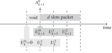
WhenU0
k =0, there is no packet ready for transmission at thekth transmission opportunity, no transmission takes place, hence the creation of a void is unavoidable. The next transmission opportu-nity occurs at the end of this void slot. Therefore, the queue con-tents at consecutive transmission opportunities relate as,
Uk0+1=Uk1+A0k+1,
Uki+1=Uki+1 fori=1,...,d−2,
Ukd+−11=0. (3) The relation between the different random variables is also visu-alised in figure 3, again ford=3.
The former set of system equations further reveals an uncanny equiv-alence with polling system dynamics. Indeed, in polling terminol-ogy, all packets that have the same offset reside at the same station. As the transmission time equals the delay in a fibre loop, all these packets can be sent without the creation of voids. This means that the server remains at the same station till there are no more packets. We have an exhaustive polling system. When there are no packets left, a single-slot void is created. In polling terminology there is a single-slot switch-over time to the next station. At the next sta-tion, the server then serves until there are no more packets and then moves again, etc.
2.3
Probability generating functions
From the equivalence with an exhaustive polling system, the queue-ing system is stable provided that,
ρ=. λE[B]S<1.
In this case, there exists a stationary distribution of the queue con-tent at transmission opportunities. LetUibe the queue content at offsetiat a transmission opportunity in a stationary regime. The joint probability generating function of the queue content at trans-mission opportunities is denoted by,
F(z0,z1,...,zd−1) =E
d−1
∏
i=0
zUii
.
In view of the system equations (2) and (3), this joint probability generating function satisfies the functional equation,
F(z0,z1,...,zd−1) =F(0,z0,...,zd−2)A(z0)
+F(z0,z1,...,zd−1)−F(0,z1,...,zd−1)
z0
d−1
∏
i=0
A(zi), (4)
where the first term of the right-hand side corresponds to the event that there is no packet ready for transmission at the service instance. The second term represents the event that there is a packet ready for transmission. Next, we implicitly define the joint generating functionχas follows:
χ(z1,...,zd−1) =A(χ(z1,...,zd−1))
d−1
∏
i=1
A(zi). (5)
It is not hard to see thatχis the joint probability generating func-tion of the number of arrivals at the different offsets from the present slot (excluding offset 0) during a so-called sub-busy period, which is the time needed to reduce the queue content at offset 0 by one. This notion stems from the observation that during a packet trans-mission, the number of arrivals at the offsets other than 0 equals ∏d−1
i=1A(zi). However, during the last slot of a packet transmission, a number of packet arrivals, which is represented by the probabil-ity generating functionA(·), occurs at offset 0. The queue content
at offset 0 will not have been effectively reduced by one, how-ever, before each of these packets are transmitted too. As these packet transmissions themselves each lead to a number of arrivals at the other offsets that is represented by the probability generating functionχ(z1,...,zd−1), the total contribution from these arriving
offset-0 packets is given byA(χ(z1,...,zd−1)).
By substitutingz0=χ(z1,...,zd)into (4) and by solving for the partial generating functionF(0,z1,...,zd−1), we obtain the
follow-ing functional equation for this generatfollow-ing function,
F(0,z1,...,zd−1) =
F(0,χ(z1,...,zd−1),...,zd−2)A(χ(z1,...,zd−1)). (6)
Equations (4), (5) and (6) and the moment generating property al-low for calculating all moments of the number of customers at the different offsets on transmission opportunities. These can then in turn be used to obtain moments of the queue content at departure epochs, arrival epochs and random slot boundaries as can be seen from the following arguments.
Let a start instant be a slot boundary where a transmission effec-tively starts. Clearly, a start instant is a transmission opportunity
where the queue content at offset 0 is non-zero. Therefore, the probability generating function of the queue content (irrespective of the offset) at start instants equals,
Us(z) =F(z,z,...,z)−F(0,z,...,z) 1−F(0,1,...,1) .
As a service starts at an actual transmission, there is a departured
slots away. Hence the probability generating function of the queue content at departure instants equals,
Ud(z) =Us(z)
A(z)d
z
The generating function of the queue content at arrival instants
Ua(z)and at departure instantsUd(z)are equal, if arrivals and de-partures occur one by one. This result does not hold in the current batch arrival setting. However, without imposing any extra restric-tions, we may assume that the arrivals within a batch are ordered. The arguments that show equality of the distributions at departure and arrival instants, then also hold in the batch arrival setting pro-vided that the queue content as seen by an arrival also includes all arrivals within the batch that have a lower order.
Finally the queue content at arrival instants as defined above re-lates to the queue content at random slot boundaries by applying the classic inspection time paradox. The queue content at arrival instants is the sum of the queue content at random slot boundaries and the number of simultaneous arrivals, that have a lower order. In view of these arguments, we find,
Ur(z)
A(z)−1
A(1)(z−1)=Ua(z) =Ud(z),
whereUr(z)is the probability generating function of the queue con-tent at random slot boundaries.
In view of the expressions above, it only remains to apply the ment generating property of generating functions to obtain the mo-ments of the queue content at random slot boundaries. First, thenth order partial derivatives ofχevaluated inz1=z2=...=zd−1=
1 can be retrieved by evaluating thenth order partial derivatives of the functional equation (5) inz1=z2=...=zd−1=1.
In-deed, these derivatives yield a system of equations that allows one to solve for thenth order partial derivatives and express these in terms of lower order derivatives. Hence, all partial derivatives of χ inz1=z2=...=zd=1 can be obtained recursively. Sec-ondly, the partial derivatives of the functional equation (6) inz1=
z2=...=zd=1 can be likewise expressed in terms of the partial derivatives ofχ. Finally, solving (4) forF(z0,z1,...,zd)expresses
F(z0,z1,...,zd−1)in terms ofF(0,z1,...,zd−1). Hence, the
par-tial derivatives ofF(z0,z1,...,zd−1)inz0=z1=...=zd=1 are easily obtained. After tedious but straightforward calculations the following expressions for the mean and the variance of the queue content at random slot boundaries are obtained:
E[Ur(d)] =
d
2
E[A] (1−E[A]) +Var[A]
1−dE[A] , (7)
and,
Var[Ur(d)] =d 3
E[A3]
1−dE[A]+ d2
4
Var[A]2
(1−dE[A])2
+dVar[A] 12
6−24 E[A] +20 E[A]2
(1−E[A])(1−dE[A])2
+d2Var[A]E[A] 12
−(6−18 E[A] +17 E[A]2) +4 E[A]d−E[A]2d2
(1−E[A])(1−dE[A])2
+dE[A] 12
E[A]2d2−4 E[A]2−3dE[A] +2
1−dE[A] . (8)
HereAdenotes the number of arrivals at a random slot boundary, which has generating functionA(z).
2.4
Back to the asynchronous queueing model
With the expressions for the moments in the discrete setting estab-lished we return to the continuous-time model. Recall thatA(z)
was defined in terms of the continuous-time arrival process in (1). Hence, the mean and variance and third-order moment ofAequals,
E[A] =E[B]λS
d , Var[A] =E[B
2]λS
d , (9)
and,
E[A3] =λS d E[B
3] +
3λ
2S2
d2 E[B]E[B 2] +λ3S3
d3 E[B] 3.
(10)
Plugging the former expressions into (7) and (8) and taking the limitd→∞, yields the following expressions for the mean and
variance of the queue content at random time instants:
E[Ur] =ρ 2
E[B] +E[B2]
E[B](1−ρ),
and,
Var[Ur] = ρ
2E[B2]2
4(1−ρ)2E[B]2−
ρ(ρ3−4ρ2+6ρ−6)E[B2]
12(1−ρ)2E[B]
+ρ
12(2−ρ) +
E[B3]ρ
3(1−ρ)E[B].
In the absence of batches, that isB=1 with probability 1, the for-mer expressions further simplify to the surprisingly and intrigu-ingly simple expressions,
E[Ur] = ρ
1−ρ, (11)
and,
Var[Ur] =ρ 6
4−ρ (1−ρ)2+
ρ 6(2−ρ).
Note that the load in the absence of batches isρ=λS. Remarkably, the mean queue content is the same as in anM/M/1 queue with the same load and twice the size of the queue content in anM/D/1 queue! From the former expressions, we see that mean and variance of the queue content only depend on the load and not on the packet lengthSin the absence of batches. Moreover, this is also the case for the discretised system as can be seen from equations (9) and (10).
0.0 0.2 0.4 0.6 0.8 1.0 ρ
0 2 4 6 8 10
E[
U
(
d
)
r
]
d= 1
d= 5
d=∞
(a) Mean queue content
0.0 0.2 0.4 0.6 0.8 1.0
ρ
0% 10% 20% 30% 40% 50%
φE
(
d
)
d= 1 d= 5
(b) Discretisation gain
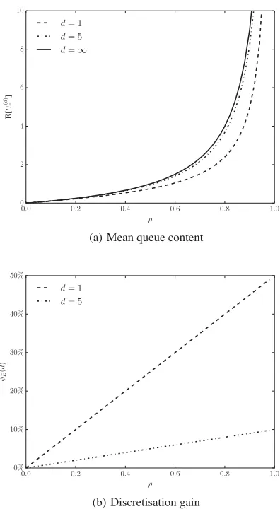
Figure 4: Mean queue content versus the loadρ (a) and the corresponding discretisation error (b) for different values ofd
and for the asynchronous queue (d=∞).
3.
NUMERICAL EXAMPLES
In this section, we first consider the link between the discrete and the continuous system, with figures 4 and 5, to then highlight the impact of the scheduling discipline, in figure 6.
Figures 4(a) and 5(a) show the mean and variance versus the load ρfor two values of the discretisation parameterdand for the asyn-chronous system. For the discrete system, the batch sizeBfollows a Poisson distribution; for the asynchronous system withd=∞, batch sizes are reduced to 1 (B=1), with single arrivals. In view of the remarks at the end of the previous section, any packet lengthS
can be assumed. The figures immediately reveal that discretisation improves performance. This is not unexpected as all arrivals within a slot are postponed until the end of the slot, and the transmission of arrivals at equal offset takes place uninterruptedly, with voids of zero length in between. For better comparison between the discre-tised and asynchronous systems, we depict the discretisation gain in figures 4(b) and 5(b) for the mean and variance, respectively. The discretisation gain of the meanφE(d)and of the varianceφV(d)are
0.0 0.2 0.4 0.6 0.8 1.0 ρ
0 5 10 15 20
Var[
U
(
d
)
r
]
d= 1
d= 5
d=∞
(a) Variance of the queue content
0.0 0.2 0.4 0.6 0.8 1.0
ρ
0% 10% 20% 30% 40% 50%
φV
(
d
)
d= 1 d= 5
(b) Discretisation gain
Figure 5: Variance of the queue content versus the loadρ(a) and the corresponding discretisation error (b) for different val-ues ofdand for the asynchronous queue (d=∞).
defined as,
φE(d) =E[
Ur]−E[Ur(d)] E[Ur]
100%, and,
φV(d) =Var[
Ur]−Var[Ur(d)] Var[Ur] 100%.
As can be understood from the figures, the gap between the discrete and continuous model is very limited for low values of the load, both for the mean value as the variance of the queue content. For high traffic load, the difference is substantially larger, especially ford=1, where it amounts to up to 50%. For higher values ofd, however, the gap is much lower, amounting to no more than 10% ford=5 for the entire range of the load.
Next, we focus on the influence of the scheduling discipline, con-trasting the proposed VAS with classic FCFS in terms of sojourn time or waiting time, i.e., the mean time elapsed between moment of arrival and departure. We assume an asynchronous setting with
0.0 0.2 0.4 0.6 0.8 1.0 ρ
0 20 40 60 80 100
E[
W
]
FCFS VAS
(a) Mean waiting time
0.0 0.2 0.4 0.6 0.8 1.0
ρ
0% 50% 100% 150% 200%
θ
(b) FCFS cost
Figure 6: Mean waiting time versus the loadρ for VAS and FCFS (a) and the relative costθfor FCFS (b).
single arrivals and a Poisson arrival process. The mean waiting time under VAS is obtained easily from the mean queue content (11) by Little’s law, as
E[WVAS] =
S
1−ρ.
The mean waiting time for FCFS is derived for a different (but, in terms of waiting time, equivalent) setting in [17], and reads
E[WFCFS] =
S
2−exp(ρ).
As suggested by this formula, the critical load under FCFS schedul-ing is not 1 but rather a smaller value, equal to ln(2). To compare both, we choose a valueS=10, resulting in figure 6(a). Clearly, the difference between the two scheduling disciplines is negligible as long as the load is (very) low. This quickly changes for intermedi-ate to high load, with a much larger waiting time for FCFS than for VAS, and a final ‘split’ when the critical load for FCFS is reached (displayed as a vertical dashed line atρ=ln(2)). To get a better view on the difference, we also consider the relative cost of FCFS
scheduling instead of VAS, by a cost parameterθ, defined as θ=E[WFCFS]−E[WVAS]
E[WFCFS]
100%.
Figure 6(b) sets outθas a function of the load. As can be seen from the definition ofθ, the cost (and thus, the figure) is independent of
S. The figure confirms the qualitative observation of 6(a), with a cost reaching 200% as load increases to about 60%. Clearly, VAS outperforms FCFS by far in the given system, due to the effective mitigation of voids between outgoing packets, avoiding voids.
4.
CONCLUSIONS
This paper provides an exact performance analysis for optical fibre-loop buffers with a void-avoiding schedule, in which packets find-ing the outgofind-ing channel available upon arrival are transmitted im-mediately. Key to our performance analysis was an auxiliary time-discretisation step which, rather unexpectedly, transformed the fibre-loop queueing system into an exhaustive polling system. By letting the slot length approach 0, we obtained the moments of the queue content of the fibre-loop buffer. The formulas for the mean queue content are surprisingly simple. In particular, in the absence of batch arrivals, the mean queue content equals the mean queue con-tent of an equally loadedM/M/1 queue.
Acknowledgements
The research of the second author was performed when visiting Ghent University in the context of the IAP Bestcom project funded by the Belgian government, while being a PhD student funded in the framework of the STAR-project “Multilayered queueing systems’ by the Netherlands Organisation for Scientific Research (NWO). The first author is a postdoctoral fellow with the Science Foundation, Flanders (FWO-Vlaanderen). This research was par-tially funded by the Interuniversity Attraction Poles Programme initiated by the Belgian Science Policy Office.
5.
REFERENCES
[1] E. Altman and D. Fiems. Expected waiting time in symmetric polling systems with correlated walking times.
Queueing Systems, 56(3–4):241–253, 2007.
[2] M. A. A. Boon, R. D. van der Mei, and E. M. M. Winands. Applications of polling systems.Surveys in Operations Research and Management Science, 16:67–82, 2011. [3] O. J. Boxma and W. P. Groenendijk. Pseudo-conservation
laws in cyclic-service systems.Journal of Applied Probability, 24:949–964, 1987.
[4] E. F. Burmeister, D. J. Blumenthal, and J. E. Bowers. A comparison of optical buffering technologies.Optical Switching and Networking, 5(1):10–18, 2008.
[5] F. Callegati. Optical buffers for variable length packets.IEEE Communications Letters, 4(9):292–294, 2000.
[6] S. N. Fu, P. Shum, L. Zhang, C. Q. Wu, and A. M. Liu. Design of SOA-based dual-loop optical buffer with a 3x3 collinear coupler: Guideline and optimizations.Journal of Lightwave Technology, 24(7):2768–2778, 2006.
[7] V. Kavitha and E. Altman. Continuous polling models and application to ferry assisted WLAN.Annals of Operations Research, 198(1):185–218, 2012.
[8] Dirk P. Kroese and Volker Schmidt. A continuous polling system with general service times.The Annals of Applied Probability, 2(4):906–927, 11 1992.
[9] Dirk P. Kroese and Volker Schmidt. Single-server queues with spatially distributed arrivals.Queueing Systems, 17(1-2):317–345, 1994.
[10] D.P. Kroese and V. Schmidt. Queueing systems on a circle.
ZOR – Methods and Models of Operations Research, 37:303–331, 1993.
[11] R. Langenhorst, M. Eiselt, W. Pieper, G. Grosskopf, R. Ludwig, L. Kuller, E. Dietrich, and H.-G. Weber. Fiber loop optical buffer.Journal of Lightwave Technology, 14:324–335, 1996.
[12] H. Levy and M. Sidi. Polling systems: Application, modeling and optimization.IEEE Transactions on Communications, 38:1750–1760, 1990.
[13] A. M. Liu, C. Q. Wu, M. S. Lim, Y.D. Gong, and P. Shum. Optical buffer configuration based on a 3×3 collinear fiber coupler.Electronics Letters, 40(16):1017–1019, 2004. [14] C. Mack. The efficiency ofNmachines uni-directionally
patrolled by one operative when walking time is constant and repair times are variable.Journal of the Royal Statistical Society Series B, 19:173–178, 1957.
[15] C. Mack, T. Murphy, and N. L. Webb. The efficiency ofN
machines uni-directionally patrolled by one operative when walking time and repair times are constants.Journal of the Royal Statistical Society Series B, 19:166–172, 1957. [16] J. A. C. Resing. Polling systems and multitype branching
processes.Queueing Systems, 13:409–426, 1993.
[17] W. Rogiest, J. Lambert, D. Fiems, B. Van Houdt, H. Bruneel, and C. Blondia. A unified model for synchronous and asynchronous FDL buffers allowing closed-form solution.
Performance Evaluation, 66(7):343 – 355, 2009.
[18] L. Rojas-Nandayapa, S. Foss, and D. P. Kroese. Stability and performance of greedy server systems.Queueing Syst. Theory Appl., 68(3-4):221–227, August 2011. [19] A. Rostami and S. S. Chakraborty. On performance of
optical buffers with specific number of circulations.IEEE Photonics Technology Letters, 17(7):1570–1572, 2005. [20] H. Takagi. Analysis and application of polling models. In
G. Haring, C. Lindemann, and M. Reiser, editors,
Performance Evaluation: Origins and Directions, volume 1769 ofLecture Notes in Computer Science, pages 423–442. Springer Berlin Heidelberg, 2000.
[21] T. Tanemura, I. M. Soganci, T. Oyama, T. Ohyama, S. Mino, K. A. Williams, N. Calabretta, H. J. S. Dorren, and Y. Nakano. Large-capacity compact optical buffer based on inp integrated phased-array switch and coiled fibre delay lines.Journal of Lightwave Technology, 29(4):396–402, Feb 2011.
[22] C. Y. Tian, C. Q. Wu, G. N. Sun, X. Li, and Z. Y. Li. Quality improvement of the dual-wavelength signals in DLOB via power equalization.Optoelectronics Letters, 4:361–364, 2008.
[23] K. Van Hautegem, W. Rogiest, and H. Bruneel. Void-creating algorithm in ops/obs: mind the gap. InProceedings of ICNAAM 2014, number 3–4, pages 1–4, 2014.
[24] Y.J. Wang, C. Q. Wu, Z. Wang, and X. J. Xin. A new large variable delay optical buffer based on cascaded double loop optical buffers (DLOBs). InProceedings of the Optical Fibre Communication (OFC) conference, pages 1–3, 2009.