©2013 JNAS Journal-2013-2-S3/1054-1063 ISSN 2322-5149 ©2013 JNAS
Simulation and Performance Assessment
between hybrid algorithms CACO and
SVR-CGA to more accurate predicting of the pipe
failure rates
Moosa Kalanaki
1and Jaber Soltani
2*1. Master Degree in Artificial Intelligence, Aboureyhan Campus, University of Tehran, Iran 2. Assistant Professor of Irrigation and Drainage Engineering Department, Aboureyhan Campus,
University of Tehran, Iran
Corresponding author: Jaber Soltani
ABSTRACT: Nowadays many studies have been done for prediction pipe failure rates in urban and other places, each of them with effective parameters has own features. So, managers and those responsible for these systems should have a more accurate and real knowledge of the structural failures and breakage in the main water supply pipes. Several studies and methods have been introduced for predicting failure rates in urban water distribution network pipes by researchers, each of them has some special features regarding the effective parameters and many methods such as Classical and Intelligent methods are used, leading to some improvements. In this paper, effective parameters for predicting water distribution network are taken into two models (Hybrid SVR-CACO and SVR-CGA) and are compared with each other, an analysis and comparison of various types of kernel and loss functions is performed for SVM. This research is aimed at optimizing related parameters to SVM and selecting the optimal model of SVM for better pipe failure rate prediction by CACO and CGA.
Keywords: Support vector regression, Continuous ant colony algorithm, Continuous genetic algorithm, Kernel functions, Pipe failure rates
INTRODUCTION
One of the main objectives of efficient management and optimal operation of urban water distribution network is to present a model for predicting breakages of urban water distribution networks. This leads to achieving some goals such as supplying sanitary potable water of a high quality and quantity as required Accordance with WHO standards, reducing the waste of water caused by breakages as well as lowering the repair, maintenance and rehabilitation costs.
To achieve the mentioned objectives, In the first stage events and factors influence in water distribution networks must be considered and the effects of pipeline characteristics on failures of pipes be determined so as to reduce the number of accidents through correct and targeted policy-making, and as a result more precisely predict the pipe breakage rates in distribution systems and take necessary actions for preventing them.
1055
A model introduced that associated breakage factor with age. They presented an exponential model for predicting pipe failure rates (Shamir and Howard, 1979).
In another study with comparing among NLR, ANN and ANFIS methods with some effective parameters results of the comparisons indicated that ANN and ANFIS methods are better predictors of failure rates compared with NLR. The results of the comparison between ANN and ANFIS showed that ANN model is more sensitive to pressure, diameter and age than ANFIS; So, ANN was more reliable (Tabesh et al., 2009).
SVM techniques used non-linear regression for environmental data and proposed a multi-objective strategy, MO-SVM, for automatic design of the support vector machines based on a genetic algorithm. MO-SVM showed more accurate in prediction performance of the groundwater levels than the single SVM (Giustolisi, 2006).
Pressure sensitive and EPANET was used for estimating and Hydraulic modeling. EPANET results were used as SVM inputs. Research results showed that the leakage rate is predictable and the smallest changes are predictable using the employed sensors (Mashford, 2009).
A prediction model of the pipe break rate was first developed using genetic programming. which minimizes the annual cost of break repair and pipe replacement. Finally, the optimal pipe replacement time was determined by the model (Xu et al., 2013).
Rough set theory and support vector machine (SVM) was proposed to overcome the problem of false leak detection. For the computational training of SVM, used artificial bee colony (ABC) algorithm, the results are compared with those obtained by using particle swarm optimization (PSO).Finally; obtained high detection accuracy of 95.19% with ABC (Mandal et al., 2012).
In this paper, combined ANN and GA model has been used to determine the effective parameters in pipe failure rates in water distribution system using the combination of ANN and GA. ANN model was developed in order to related parameters of breakage with pipe failure rates. The results lead to minimize the simultaneous error rates (Soltani and Rezapour Tabari, 2012).
In this paper, effective parameters in predicting pipes failure rate of water distribution network are taken into two models Hybrid SVR-CACO and SVR-CGA compared with them, an analysis and comparison of various types of kernel and loss functions is performed for SVR. This research is aimed at optimizing parameters related to SVR and selecting the optimal model of SVR for better pipes failure rate prediction by CACO and CGA algorithms So in this research compared hybrid SVR-CGA and SVR-CACO models to predict pipe failure rates in water distribution networks to reduce the number of events. By comparing these results with the other methods such as ANFIS, ANN, and ANN-GA that had been done in the past results show the SVR-CACO model has better performance than the other models especially in time elapse. Also, with combining SVR and CGA obtained better parameters proportional to the data type and the model shows better performance in accuracy.
MATERIALS AND METHODS
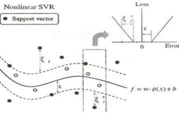
Support vector machines (SVMs) are learning machines which implement the structural risk-minimization inductive principle to obtain a good generalization on a limited number of learning patterns (Gonzalez-Abril et al., 2011). Support vector machine is an algorithm to maximize a mathematical function based on data sets. To create maximum margin, at first two adjacent parallel planes and a separator is designed. They get away from each other until they hit the data. The plane farthest from the others is the best separator (Carrizosa& Romero Morales, 2013). Support vector machine regression (SVR) is a method to estimate the mapping function from Input space to the feature space based on the training dataset (Vapnik, 1992).
In the SVR model, the purpose is estimating w and b parameters to get the best results. w is the weight vector and b is the bias, which will be computed by SVM in the training process.
In SVR, differences between actual data sets and predicted results is displayed by ε. Slack variables are (ξi, ξi∗ ) considered to allow some errors that occurred by noise or other factors. If we don’t use slack variables, some errors may occur, and then the algorithm cannot be estimated. Margin is defined as margin=‖w1‖. Then, to maximize the margin, through minimizing ‖w‖2, the margin becomes maximized. These operations give in Equations (1- 3) and these are the basis for SVR (Vapnik, 1992).
Minimize 1 2||w||
2+C∑ ξ i n i=1 +ξi
* (1)
subject to : yi(wTx
1056
C is a parameter that determines the tradeoff between the margin size and the amount of error in training and ξi, ξi* are slack variables.
2.1. Kernel Functions
The basic idea of mapping input variable to the higher dimensional space is for easier separation by linear functions. Because it is difficult and more costly to work with high dimensional feature space, so we use feature space. A kernel function is a linear separator based on inner vector products and is defined as Equation. (4):
𝑘(𝑥𝑖, 𝑥𝑗) = 𝑥𝑖𝑇𝑥𝑗 (4) If the data points are moved using φ: x → φ(x) to the feature space (higher dimensional space), their inner products turn into Equation. (5) (Qi et al., 2013).
k(xi,xj)=φ(xi)T.φ(xj) (5) xi is the support vectors and xj is the training data.
Kernel functions are equivalent to inner product in the feature space. Thus, instead of doing costly computing in feature space, we use kernel functions (Hofmann et al.,2008). Nonlinear kernel functions give more linear separable ability to the feature space; in the other words, we add so much to the dimensions that data are separated in a linear form.
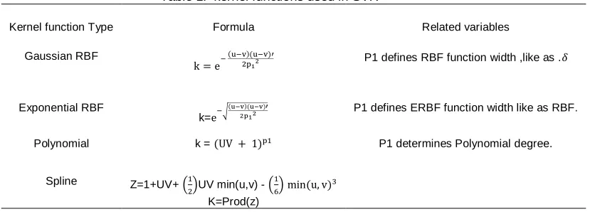
The most important kernel functions and the related parameters are included in Table 1, where U and V are training and test data respectively.
Table 1. kernel functions used in SVR
Related variables Formula
Kernel function Type
P1 defines RBF function width ,like as .𝛿 k = e−
(u−v)(u−v)′ 2p12
Gaussian RBF
P1 defines ERBF function width like as RBF. k=e−√
(u−v)(u−v)′ 2p12
Exponential RBF
P1 determines Polynomial degree. k = (UV + 1)p1
Polynomial
Z=1+UV+ (1
2)UV min(u,v) - ( 1
6)min (u, v) 3
K=Prod(z) Spline
αi is the vector of Lagrange multipliers and represent support vectors. If these multipliers are not equal to zero, they are multipliers; otherwise, they represent support vectors (Vapnik and Chapelle, 2000).
Here, w is equal to Equation. (6).
w=∑ (i αi-α̅i)xi (6) Accordingly, the SVR function F(x) becomes the following function.
F(x)=∑ (i=1 α̅ι-αi)K(xi,x)+b (7) Equation. (7) can map the training vectors to target real values, while allowing some errors. To minimize errors and minimize risks, the goal is to find a function that can minimize risks, Equation. (8).
Remp[f]=1
l∑li=1c(xi,yi,f(xi)) (8)
𝑐(𝑥𝑖, 𝑦𝑖, 𝑓(𝑥𝑖)) , denotes a cost function determining how the estimation error will be penalized based on empirical data X. Remp represents empirical risks. While dealing with a few data in very high dimensional spaces, this may not be a good idea, as it will lead to over-fitting and thus bad generalization properties. Hence, one should add a capacity control term, which in the SV results is to be ‖w‖2 and leads to the regularization of risk function (Smola and Scholkopf, 1998).
1057
Figure 1. ε-insensitive loss function
A Loss function implies to ignore errors associated with points falling within a certain distance. If ε-insensitive loss function is used, errors between -𝜀 and +𝜀 are ignored. If C=Inf is set, regression curve will follow the training data inside the margin determined by 𝜀 (Smola and Scholkopf, 1998). The related equation is shown in Equation. (10).
|ξ|ε={0 if | |ξ|≤ε
ξ|- ε otherwise. (10) The quadratic loss function Fig.2 drives the proximal hyper plane close enough to the class itself, and it penalizes every error (Qi et al., 2013). If quadratic loss function is used, memory requirements will be four times less than ε-insensitive loss function (Gunn, 1998).
Figure 2. quadratic loss function
3. Searching Algorithms
Generally so far, the previous researches have appropriated SVM parameters obtained by trial and error. In the trial and error method, each parameter is tested to approach the appropriated values. However, this method has very time-consuming and is not sufficiently accurate.
Therefore, in this study integrated models compare and proposed to search for the possible solutions. As it noted, using the trial and error method is suitable for simpler and easier problems, but is not prone for complex ones of higher dimensional space, because it takes more time and ultimately might not converge to the solution. Therefore, due to the higher dimensions of the problem and the number of data, the integrated models were considered. Also, intelligent searching models have a high capability and suitable performance related to this problem; so, these algorithms were selected. In this study, search doing in practical solution with intelligent searching algorithms and the best of them selected for choosing an optimal SVR structure. Considering the fact that the parameters used in SVR and corresponding parameters are continuous in the solution Space, Continuous GA and Continuous ACO had been used, because when the variables are continuous, it is more logical to represent them by floating-point numbers.
3.1. Continuous ANT colony
The Ant colony optimization algorithm is an optimized technique for resolving computational problems which can be discovered good paths. The process by which ants could establish the shortest path between ant nests and food. Initially, ants leave their nest in random directions to search for food.
This technique can be used to solve any computational problem that can be reduced to finding better paths in a graph these formulas have been shown in Equations. (11) and (12). This method had been chosen from (Hong et al., 2011) paper.
Pk(i,j)={ {[τ(i,s)]
α[η(i,s)]β sϵMk
arg max
, if q≤q0
1058
Pk(i,j)={
[τ(i,s)]α[η(i,s)]β
∑sϵMk[τ(i,s)]α[η(i,s)]β,j∉Mk 0 O.w
(12)
where 𝜏(i, j) is the pheromone level between node i and node j, 𝜇(i, j) is the inverse of the distance between nodes i and j. In this study, the forecasting error represents the distance between nodes. The 𝛼 and 𝛽 are parameters determining the relative importance of pheromone level and Mk is a set of nodes in the next column of the node matrix for ant k. q is a random uniform variable [0, 1] and the value q0 is a constant between 0 and 1, i.e., q0 𝜖[0, 1]. The local and global updating rules of pheromone are expressed as Equation. (13) and (14), respectively
τ(i,j)=(1-ρ) τ(i,j)+ρτ0 (13) τ(i,j)=(1-δ)τ(i,j)+δΔτ(i,j) (14) The δ is the global pheromone decay parameter, 0 <δ< 1, and, based on authors’ experiments.
The Δ (i, j), expressed as Equation. (15), is used to increase the pheromone on the path of the solution
Δτ(i,j) ={
1
L , if (i,j)ϵglobalbest route
0 O.W (15) where L is the length of the shortest route.
At first to get SVR related parameters, each parameters show by 10 nodes, so the range of numbers limited between [0, 9]. For getting more accurate computed parameters 5 numbers considered.
The values ρ of and τ0 are set to be 0.2 and 1, respectively. Assume the limits of parameters σ, C, and ε are 1, 100,000, and 1, respectively. Numbers of nodes for each ant set to 50, so total nodes are equal to 150.
3.2. Continuous Genetic Algorithm
The continuous GA is inherently faster than the binary GA, because the chromosomes do not have to be decoded prior to the evaluation of the cost function (Haupt and Haupt, 2004). Thus, using the aforementioned variables like kernel parameters as decision variables in a population-based optimization strategy may be a way of constructing an optimal SVR. To cover the entire search space, the initial population was considered randomly, commensurate with the best fitness function Equation. (16) of each population; the best of them has been selected. Some properties of GA, such as the ability of solving hard problems, noise tolerance, easy to interface and hybridize, make them a suitable and quite workable technique for parameter identification of fermentation models (Angelova and Atanassov, 2012).
Minimize cost:|Y̅pred-Ytrain| (16)
1059
Figure 3. The proposed SVR-CGA and CACO-SVR hybrid system which predict the pipe failure rates
In this research, the selection rate is considered at 0.5; thus, the chromosomes must be firstly sorted by their fitness functions and half of the best population is selected for the next generation. The single point Crossover rate has been considered and mutation rate selected between 0.1 and 0.2 based on its kernel function type. This research has been developed by MATLAB (version 7.12(R 2011a)) and SVM Toolbox and parameters were localized by Continues GA to solve these problems. Equation. (17) is used for normalizing the Input values to the models.
xn=0.8 (x-xmin)
(xmax-xmin)+0.1 (17) x is the original value ,x min is the minimum value and x max is the maximum value between input values, and x n shows normalized values. So that, input results are between [0.1, 0.9].
Also, In this paper, the root of mean squared error (RMSE), normal root of mean squared error (NRMSE) and coefficient of determination(R 2) are used as assessment criteria of the reliability of the model.
R2 (∑ (yactual-y̅actual) n
i=1 (ypred-y̅pred)) 2
∑ni=1(yactual-y̅actual)2∑ni=1(ypred-y̅pred)2
(18)
𝑅𝑀𝑆𝐸 = √ 1
𝑛∑ (𝑦𝑎𝑐𝑡𝑢𝑎𝑙𝑖− 𝑦𝑝𝑟𝑒𝑑𝑖)
2
𝑛
𝑖=1 (19) NRMSE= RMSE
var(yactual) (20)
Where yactual is the observed data, yprediction is the predicted data, yaverage is the average of data and n is the number of observations. Also, var(y actual) is the variance of actual data.
4. Case Study
1060
Figure 4. Schematic of study area and pressure measurement points
In order to failure rate modeling of the asbestos cement pipes, the daily events recorded in the 2005 to 2006 years over 2438 record data such as diameter, year of implementation ,installation depth, total accident happens and the average of hydraulic pressure. These data have been collected from local water and water waste company.
RESULTS AND DISCUSSION
Input parameters to the combined SVR-CACO and SVR-CGA models included installation depth, pressure, age, length, and diameter and the output parameter model base on predicted output values from the training input values. Calculated variables to appropriate the best values of the kernel functions based on the best type of loss is as follows:
1- According to ε-insensitive function that consists of the effective parameters of kernel function (ε, C). 2- According to quadratic loss function that consists of the effective parameters of kernel function (C).
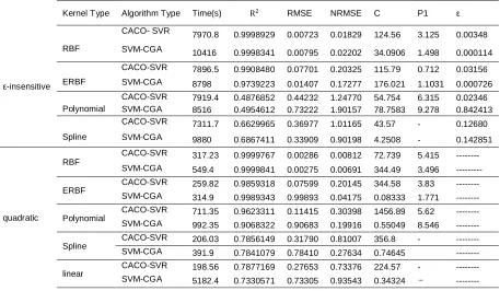
The results obtained by mentioned algorithms and appropriate kernel and loss functions have been shown in Table 2.
According to the above results, quadratic loss function shows better results in time and other parameters than ε-insensitive in Table 2.
ε P1 C NRMSE RMSE R2 Time(s) Algorithm Type Kernel Type 0.00348 3.125 124.56 0.01829 0.00723 0.9998929 7970.8 CACO- SVR RBF ε-insensitive 0.000114 1.498 34.0906 0.02202 0.00795 0.9998341 10416 SVM-CGA 0.03156 0.712 115.79 0.20325 0.07701 0.9908480 7896.5 CACO-SVR
ERBF SVM-CGA 8798 0.9739223 0.01407 0.17277 176.021 1.1031 0.000726
0.02346 6.315 54.754 1.24770 0.44232 0.4876852 7919.4 CACO-SVR
Polynomial SVM-CGA 8516 0.4954612 0.73222 1.90157 78.7583 9.278 0.842413
0.12680 - 43.57 1.01165 0.36977 0.6629965 7311.7 CACO-SVR
Spline SVM-CGA 9880 0.6867411 0.33909 0.90198 4.2508 - 0.142851
--- 5.415 72.739 0.00812 0.00286 0.9999767 317.23 CACO-SVR RBF quadratic --- 3.496 344.49 0.00691 0.00275 0.9999841 549.4 SVM-CGA --- 3.83 344.58 0.20145 0.07599 0.9859318 259.82 CACO-SVR ERBF --- 1.771 0.08333 0.04175 0.99893 0.9989343 314.9 SVM-CGA --- 5.62 1456.89 0.30398 0.11415 0.9623311 711.35 CACO-SVR Polynomial --- 8.546 0.55049 0.19916 0.90683 0.9068322 992.35 SVM-CGA --- - 356.8 0.81007 0.31790 0.7856149 206.03 CACO-SVR Spline --- 0.74645 0.27634 0.78410 0.7841079 391.9 SVM-CGA --- - 224.57 0.73376 0.27653 0.7877169 198.56 CACO-SVR linear --- 0.34324 0.93543 0.73305 0.7330571 5182.4 SVM-CGA
1061
Comparing results between Hybrid SVR-CACO and SVR-CGA models has been shown in Fig.5, time considered as a comparison parameter. By over looking at Table 2 and Fig.5 can be found CACO searching algorithm has a better performance in time-consuming than the CGA.
Figure 5. comparing between Hybrid SVR-ACO and SVR-CGA models time
Results in Table 2 shows the correlation and estimation of error in the RBF kernel has an excellent performance relative to the other kernel functions also by comparing the results in Table 2, shows quadratic loss function present a better result than ε-insensitive loss function.
Results from ε-insensitive loss function and related kernel functions present in Fig. [6-8].
Figure 6. Results by Poly kernel function and loss
function Figure 7. Results by RBF kernel function and loss function
According to the Figure results can be found CACO searching algorithm as same as CGA in accuracy but it has a better performance in time-consuming than the CGA. Fig. 7 shows the best prediction result than the other kernelin upper figures.
Figure 8. Results by eRBF kernel function and Quadratic Figure 9. Results by eRBF kernel function and Quadratic loss function loss function
1062
Figure 10. Results by Polynomial kernel function and Quadratic loss function
Upper Figures show the quadratic loss function performances, According to these figures our results have a better prediction and show better results than ε-insensitive loss function.
CONCULSION
In the recent decades, public health and health care has been more attention by responsible in each region. One critical infrastructure to achieve the promote public health and better quality in water according to WHO standard is the water distribution systems ready to operate and timeless through correct management and use optimized.
So in this research compared hybrid SVR-CGA and SVR-CACO models to predict pipe failure rates in water distribution networks to reduce the number of events.
The compared SVR models in order to make the relationship between the failure rate parameters in pipes with the number of events and failure of pipes considered as a main component of urban infrastructure, water supply and hygiene and health. Also by using the CGA and CACO optimal kernel function and SVR related parameters has been found.
By comparing these results with the other methods such as ANFIS, ANN, and ANN-GA that had been done in the past, results show the SVR-CACO model has better performance than the other models especially in time elapse. Also, with combining SVR and CGA obtained better parameters proportional to the data type and the model shows better performance in accuracy.
By comparing among the kernel functions RBF and eRBF offered favorable results and in the loss functions regard to quadratic time and accuracy quadratic loss function has been shown more favorable results than ε-insensitive loss function.
REFERENCES
Angelova M, Atanassov K. 2012. Purposeful model parameters genesis in simple genetic ……algorithms, Compt. & Math. App. 64:221–228.
Carrizosa E,Romero Morales D. 2013. Supervised classification and mathematical optimization,Computers & OperationsResearch. 40:150–165.
Elahi Panah NA. 1998. Subsequent water distribution networks in the country until 1400,Journal Water and Environment, 284-15.
Giustolisi O. 2006. Using a multi-objective genetic algorithm for SVM construction, Journal of Hydroinf. 8:125-139.
Gonzalez-Abril L, Velasco F, Ortega JA, Franco L. 2011 .Support vector machines for classification of input vectors with different metrics, Comp. & Math. Appl. 61:2874-2878.
Gunn S. 1998. Support vector machines for classification and regression. Technical report. School of . Electronics and Computer Science, University of Southampton.
Hofmann T, Scholkopf B, Smola A. 2008. Kernel methods in machine learning, The annals of statistics. 36:1171-1220.
Hong WC, Dong Y, Zheng F, Lai CY. 2011. Forecasting urban traffic flow by SVR with continuous ACO. J. Applied Mathematical Modeling. 35:1282–1291.
Haupt R, Haupt S. 2004. Practical Genetic Algorithms, Second Edition, John Wiley and Sons, USA.
Mashford J, Silva DD, Marny D, Burn S. 2009. An approach to leak detection in pipe networks using analysis of monitored pressure value by support vector machine, IEEE Comp. Society. 3: 534 – 539.
Mandal SK, Tiwari MK, Chan FTS. 2012. Leak detection of pipeline: An integrated approach of rough.set theory and artificial bee colony trained SVM. Expert Systems with Applications, 39: 3071–3080.
1063
Soltani, J, Mohammad Rezapour Tabari M. 2012. Determination of Effective Parameters in Pipe Failure Rate in Water Distribution System Using the Combination of Artificial Neural Networks and Genetic Algorithm, J. Water and Environment (In Persian). 83:2-15.
Smola AJ, Scholkopf B. 1998. A Tutorial on Support Vector Regression, NeuroCOLT, Royal Holloway College, University of London,.
Shamir U, Howard CDD. 1979. An analytical approach to scheduling pipe replacement. J.AWWA. 71, 24–258.
Tabesh M, Soltani J, Farmani R, Savic DA. 2009. Assessing Pipe failure Rate and Mechanical Reliability of water Distribution Networks Using Data Driven Modeling, Journal of Hydroinf (IWA)11:1-17.
Vapnik VN. 1992. Principles of risk minimization for learning theory. Advances in Neural Information Processing Sys. 4: 831-838. Vapnik VN, Chapelle O. 2000 . Bounds on error expectation for support vector machines. J. Neural .Computation. 12: 2013-2036. Xu Q, Chen Q, Ma J, Blanckaert K. 2013. Optimal pipe replacement strategy based on break rate prediction through genetic