Application of Dynamic Threshold in a Lake Ice Detection Algorithm

(1)

http://www.sciencepublishinggroup.com/j/ajrs doi: 10.11648/j.ajrs.20180602.12

ISSN: 2328-5788 (Print); ISSN: 2328-580X (Online)

Application of Dynamic Threshold in a Lake Ice Detection

Algorithm

Peter Dorofy

1

, Rouzbeh Nazari

1, *

, Peter Romanov

2

1

Department of Civil and Environmental Engineering, Rowan University, Glassboro, USA

2_{NOAA Cooperative Remote Sensing Science and Technology Center (CREST), City University of New York, New York, USA}

Email address:

*

Corresponding author

To cite this article:

Peter Dorofy, Rouzbeh Nazari, Peter Romanov. Application of Dynamic Threshold in a Lake Ice Detection Algorithm. American Journal of Remote Sensing. Vol. 6, No. 2, 2018, pp. 64-73. doi: 10.11648/j.ajrs.20180602.12

Received: July 23, 2018; Accepted: August 2, 2018; Published: August 29, 2018

Abstract:

The traditional method involved in the classification of surface types such as water, ice, and snow rely on thresholds values of spectral properties that are fixed. However, the use of daily fixed thresholds leaves a substantial number of either unclassified and/or misclassified ice and water pixels. In this study, a new dynamic threshold technique is proposed to identify and map lake ice cover in the imagery of GOES-I to P series satellites. In addition, dynamic threshold can be used as an alternative solution to Bidirectional Reflectance Distribution Function (BRDF) models. The technique has been applied using GOES-13 imager data over Lake Michigan, one of five of the Great Lakes. Nine scenes based on an hourly acquisition of a single day are used to visually sample water and ice pixels. A threshold for the visible (0.62 µm) and the reflective component of the mid-infrared (3.9 µm) is determined for each scene by the intersection of the probability distributions of the water and ice samples. The thresholds are used as decision thresholds in a binary test algorithm applied on a per-pixel basis. Both fixed threshold (single scene) and dynamic thresholds (multiple scenes) have been compared. Dynamic threshold shows a significant gain in classified pixels over fixed threshold. A preliminary quantitative assessment is introduced to evaluate the algorithm’s performance using sensitivity and specificity testing. The classification results show a sensitivity of 98% when delineating thick ice and water and 87% when delineating thick/thin ice and water. Implementing a dynamic threshold, can be used in constructing ice maps in applications that benefit from high temporal resolution imagery.

Keywords:

Lake Ice Concentration, Dynamic Threshold, GOES Imager, Remote Sensing, Shortwave Infrared, Snow Index, Geographical Information System (GIS)

1. Introduction

With the launch of GOES-16 in November 2016, a new era of remote sensing research over the North and South Atlantic basin and adjacent land masses has begun. The primary GOES-16 instrument is the Advanced Baseline Imager capable of providing high spatial and temporal resolution data in 16 bands. The remote sensing scientific and engineering community has developed various products based on this instrument including ice and snow maps [1]. This particular study is twofold. 1) Present the use of dynamic threshold in developing a sea and lake ice map [2]; 2) Promote further the use of the GOES-13 imager in snow and ice mapping [3, 4] and the potential to develop these maps using historical

imagery. It is the intention of the authors, that this work may contribute to the study of climate data in the Great Lakes region of which over 30 years of data from NOAA’s GOES program are available.

(2)

American Journal of Remote Sensing 2018; 6(2): 64-73 65

sensors for snow and ice mapping are limited to clear sky conditions. Unlike polar-orbiting satellites, the higher temporal resolution of geostationary satellites offer greater opportunity in monitoring for cloud-free conditions and pixel classification via a daily composite map of cloud-free pixels. Prior to GOES-16, the GOES imagers were limited to 5 bands, none of which were in the SWIR needed for ice mapping. However, research in the use of the mid-infrared (MIR) 3.9 µm band for snow and ice maps have been investigated through the GOES imagers [3, 4].

Ice mapping products derived from polar orbiting satellites are also limited in the use of constant threshold in their algorithms [2]. For example, an ice concentration algorithm for VIIRS uses fixed threshold for the visible (vis>0.08) and (NDSI>0.45) for ice identification [5]. A reflectance threshold, as referred to in this study, is a reflectance value shared by two dissimilar surfaces (differences in spectral properties). The ambiguity that exists when classifying these surfaces is predominantly a result of the particular viewing and illumination geometry at the time of data acquisition. For example, snow has a significantly higher albedo than liquid water (difference between albedo and reflectance will be discussed in a moment). However, when sunlight reflects off the surface of a water body at the same angle that a sensor is viewing the surface there is a significant “boost” in the reflectance of water, a phenomena known as sunglint; this can lead to classification errors while distinguishing ice from water. Ice mapping products with fixed or static thresholds that do not account for the variation in illumination geometry during the day are susceptible to these errors. Unlike polar orbiting satellites, which have low frequency of coverage offering at best a daily snapshot of the illumination geometry for a given area, geostationary satellites offer continuous coverage that allows observations across various illumination geometries. This information is useful in building a threshold that adapts to these changing lighting conditions.

The challenge for developing any surface type classification process, accounting for the ambiguity of dissimilar surfaces with overlapping spectral signatures, requires an understanding of multispectral surface reflection which depends upon both illumination and viewing direction, and is described by a particular surface’s Bidirectional Reflectance Distribution Function (BRDF). Albedo is defined as the fraction of incident radiation that is reflected by a surface. The albedo of snow and ice is dependent on the solar zenith angle, . Reflectivity of snow and ice increases with increasing [6]. Albedo differs from reflectance in that albedo is the directional integration of reflectance over all possible sun-view geometries. Albedo depends on the spectral and angular distribution of incident radiation and thus is dependent on BRDF [7]. A Lambertian surface (completely diffuse) would have a BRDF plot that is cylindrical in shape with a nearly flat top; however, the reflectance of radiation from most natural surfaces is dependent on the sun-view geometry. Work has been done on laboratory measurements of

BRDF [8], including field investigations [9] and the usefulness of these measurements in remote sensing applications. Application of laboratory measurements of BRDF on remote sensing data presents challenges including the broader scale of remote sensing instruments, complexity of physically-based BRDF models in transposing them onto remote sensing data, and the heterogeneity of land cover. These challenges have been investigated by measuring BRDF of various surface types through remote sensing instruments; including airborne [10] and geosynchronous [11] and evaluated against existing BRDF models. Today, natural surface BRDF databases exist that can be used to validate satellite sensors [10].

Dynamic threshold has been proposed in this study as an alternative to investing in a BRDF model for an ice mapping algorithm. In order to build a robust and reliable ice detection algorithm, it is necessary to properly account for the effects of the variable viewing and illumination geometry of observations. Conceptually, a dynamic threshold can be an alternative solution to accounting for these effects over the use of Bidirectional Reflectance Distribution Function (BRDF) models which mathematically correct for surface reflectance anisotropy during the classification process. As a continuation of previous work [4], which provided a preliminary evaluation of the MIR band to lake ice detection using a single threshold, the results of applying a dynamic threshold are presented in this paper. A dynamic threshold in this study is a time series of hourly reflectance thresholds based on ( ∩ ), where I is the probability of a pixel detected as ice and W is the probability of a pixel detected as water. These probabilities have been derived from hourly plots of normal distributions of ice and water pixels and applied to an ice detection algorithm that uses the mid-infrared band to delineate thick ice and water. Dynamic thresholds in the visible have been used in previous studies including ice mapping which has been demonstrated over the Caspian Sea [2] and in brightness temperature for cloud detection [12].

2. Method

(3)

Figure 1. Ice cover on Lake Michigan. Image acquired by the Moderate Resolution Imaging Spectroradiometer (MODIS) on February 28, 2015 (NASA).

2.1. Satellite Channels

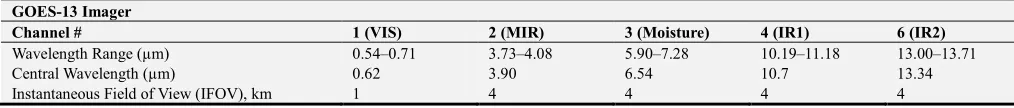
The GOES-13 satellite is in geosynchronous orbit, with a nadir located at approximately 0.05°N, 75°W. Data collected by the GOES-13 imager instrument is being used in this study. The GOES imager is a five-channel instrument (one visible, four infrared), as listed in Table 1. All channels except channel 3 are used in this study.

Table 1. GOES-13 imager channels.

GOES-13 Imager

Channel # 1 (VIS) 2 (MIR) 3 (Moisture) 4 (IR1) 6 (IR2)

Wavelength Range (µm) 0.54–0.71 3.73–4.08 5.90–7.28 10.19–11.18 13.00–13.71

Central Wavelength (µm) 0.62 3.90 6.54 10.7 13.34

Instantaneous Field of View (IFOV), km 1 4 4 4 4

2.2. Approach and Algorithm Development

The Normalized Difference Snow Index (NDSI) is a snow index measurement that has traditionally been used in delineating snow and ice from other land surface features. NDSI is the normalized difference between the 0.6 µm visible band and the 1.6 µm SWIR band. An alternative to this, for sensors not operating in the SWIR window, is the ratio of the 0.6 µm visible band and the 3.9 µm MIR band. This method is chosen since GOES-13 does not operate in the SWIR.

Thick ice and snow have relatively high reflectivity in the visible. Ice reflectance substantially increases when ice

(4)

skin temperature, and the derivation of the 3.9 µm reflection component has been implemented. Readers are encouraged to refer to that work for a detailed explanation of the pre-processing and processing procedures used in the algorithm.

As in the previous study [4], data was acquired for February 28, 2015. Acquisition times for that day were every half-hour from 1430 UTC to 2030 UTC. These are the times that GOES-13 is in the continental US (CONUS) extended scan mode with the exclusion of near 18:00 UTC which is during the time GOES-13 is operating in full disc mode. These times also correspond to daytime conditions over the eastern half of the North American continent. The mean solar zenith angle across all scenes was 56.8° with a range from 51.73° to 70.18°.

The distinction between various surface types in a satellite image becomes possible owing to their different spectral response. A threshold-based decision-tree image classification scheme is used to distinguish between water, gray ice, and thick ice. In this study, gray ice is referred to as thin or broken ice. The spectral properties of gray ice and thick ice are significantly different [4]. In this paper, R1 is referred to the

visible and R2 as the reflective component of the mid-infrared.

The R1, R2, MISI [4] thresholds were determined through a

visual inspection of the visible reflectance for a sampling of pixels from southern Lake Michigan. The sampling consists of a mix of water and ice pixels. 50 water pixels and 50 ice pixels

were identified from each acquired image. The scene images were rendered in gray scale. Cloud-free pixels relatively dark were visually classified as water, cloud-free moderately bright pixels were classified as ice. Example is shown in Figure 2. The identification of ice was visually validated against ice charts of the Great Lakes from the National Ice Center. Delineating the different ice concentrations as classified by NIC was not conducted. It should be noted that darker ice such as thin or broken ice will have reflectivity in the visible similar to water. The data is next best fitted to a normal distribution. Figure 3 are the distributions for R1, R2, and MISI at 1430,

1730, 2030 UTC. Blue is water, and red is ice. The number of bins for each distribution is equal to √ . As the sampling size was relatively small, the width of the bins is relatively wide. The R1 distributions show a clear distinction in the mean value

between water and ice. The ambiguity occurs where both distributions overlap. The overlapping indicates that a pixel has probability of being water or ice. For the scope of this paper, the point of intersection ( ∩ , where I is the probability of a pixel detected as ice and W is the probability of a pixel detected as water, is chosen as a threshold value for that particular time. All data values above this point are classified as ice and all data values below this point are classified as water. Since thick ice will have R1 values

significantly higher than water, it is reasonable to suggest that gray ice may occur at or near ∩ .

(5)

Figure 3. Probability distribution functions of water (blue) and ice (red) at 1430, 1730, 2030 UTC on February 28, 2015; (top) distribution of 0.64 µm refl; (middle) distribution of 3.9 µm refl; (bottom) distribution of MISI.

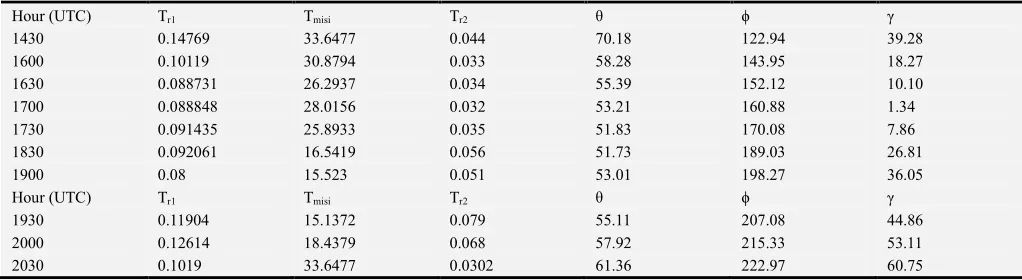
Table 2 lists the probability threshold values for R1 (Tr1), R2 (Tr2), MISI (Tmisi) for each acquisition time. Tr2 is calculated:

Tr1/Tmisi. In addition, observation geometry is also provided: solar zenith angle (θ), solar azimuth angle (ϕ), solar-satellite relative

azimuth angle (γ). The observation geometry has been calculated from a point located at 43.450°N, 87.222°W. GOES-13 azimuth and zenith angles at this location are approximately 162.22°, and 51.72° respectively.

Table 2. Probability thresholds (Tr1, Tr2, Tmisi) for individual acquisition times from population density plots for normal distributions of ice and water.

Hour (UTC) Tr1 Tmisi Tr2 θ ϕ γ

1430 0.14769 33.6477 0.044 70.18 122.94 39.28

1600 0.10119 30.8794 0.033 58.28 143.95 18.27

1630 0.088731 26.2937 0.034 55.39 152.12 10.10

1700 0.088848 28.0156 0.032 53.21 160.88 1.34

1730 0.091435 25.8933 0.035 51.83 170.08 7.86

1830 0.092061 16.5419 0.056 51.73 189.03 26.81

1900 0.08 15.523 0.051 53.01 198.27 36.05

Hour (UTC) Tr1 Tmisi Tr2 θ ϕ γ

1930 0.11904 15.1372 0.079 55.11 207.08 44.86

2000 0.12614 18.4379 0.068 57.92 215.33 53.11

2030 0.1019 33.6477 0.0302 61.36 222.97 60.75

The fixed threshold values used in the original ice mapping algorithm [4] are replaced by the threshold values from Table 2. Figure 4 shows the revised detection algorithm. Sampling cloud pixels was not conducted as it was not a goal of this

(6)

Figure 4. GOES snow/ice detection algorithm.

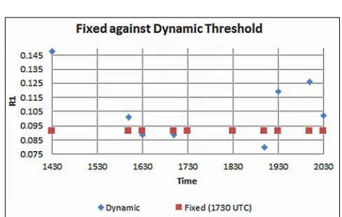
Figure 5 compares the fixed to dynamic threshold values for

R1. Fixed threshold has been selected at 1730 UTC which is

close to local solar noon [4]. There is high variability in the dynamic threshold values near the end of the day, this may be an artifact in the relatively small volume of the training data

set.

Figure 5. Fixed threshold against dynamic threshold versus acquisition times.

3. Result

Figure 6 compares the lake ice map generated for 1430 UTC at a fixed threshold (left) generated from 1730 UT (Figure 4) and dynamic threshold (right). A visual inspection reveals there are substantially less unclassified pixels.

Figure 7 is the resulting gain of classified pixels across the ten acquisition times (Table 2) for dynamic threshold over a fixed threshold. Gain is defined as the change in the number of pixels with a positive response against the same pixels tested using a static threshold (gain is zero). The most significant gains are near sunrise and sunset. Figure 8 is the final daily composite lake ice map. Application of a dynamic threshold provides less unclassified pixels, resulting in a more complete ice map.

(7)

Figure 7. Dynamic threshold pixel classification gains over fixed threshold.

Figure 8. Lake ice daily composite. (left) fixed threshold; (right) dynamic threshold.

4. Discussion

At this point, the application of dynamic threshold for this particular scene has resulted in substantially fewer unclassified pixels. The next step is to test the performance of the algorithm in its ability to delineate ice and water. The use of spatial analysis methods commonly used in Geographic Information System (GIS) has been used to quantify this performance. ESRI ArcGIS (10.2.1) is used in validating the classified pixels against Interactive Multisensor Snow and Ice Mapping System (IMS) and NIC ice maps. Vector and raster data are the two basic spatial data types used in GIS. Vector data are comprised of vertices and paths. Vertices can be used

(8)

geospatial data to be shared across multiple GIS platforms. The U.S. National Ice Center provide ice and snow products in various formats including geotiff and shapefiles. In this study, the IMS data is obtained as a geotiff and the NIC ice concentration map is obtained as a shapefile. The MISI classification data stored as a matrix in Matlab is converted to vector data for use in GIS.

There are multiple techniques in performing quantitative analysis in GIS. The process of validation in this study involves testing a MISI pixel class that satisfies a boundary

condition derived from the IMS and NIC maps that best represents the class. This decision boundary will be referred to as a catchment area. For the IMS, this is done by vectorizing the input raster. The process of vectoring a raster is shown in Figure 9. The polygons conform exactly to the raster’s cell edges (non-simplified output). This method should work well as IMS classifications are relatively homogeneous. Table 3 presents the classification scheme of this model (MISI), IMS, and NIC. The MISI values are the classes and the IMS and NIC are values of the catchment areas.

Table 3. Classification values for three products.

MISI IMS NIC (CT Codes)

2 Water 1 Water 00 Ice Free

3 Gray Ice 3 Ice 20 Young Ice

4 Snow/Thick Ice 4 Snow 91 Medium 1st Year Ice

5 Cloud 92 Fast Ice

To prepare for analysis in GIS, the classification map was down-sampled to a resolution of (4km)2/pixel. The resulting 3440 test pixels (16km2/pixel) total area of coverage is 55,040 km2 (area of Lake Michigan is approximately 58000 km2).

These 3440 test pixels that fall within the Lake Michigan boundary are spatially queried and checked for containment within each catchment area. Figure 10 shows the IMS ice catchment area in red and water catchment area in light blue (a). All MISI pixels are queried within the ice catchment (b); and within the water catchment (c). The percentage of each MISI pixel classification within each IMS catchment area are tabulated (Table 4). 2.56% remain unclassified. For the IMS product, the ice/water numerical fraction is 78.97%/20.35%; MISI product is 70.3%/12.61%.

Figure 10. (a) IMS ice catchment area in red and water catchment area in blue. Spatial query of MISI pixels within (b) IMS ice area; (c) IMS water area.

Table 4. Percentage of MISI classified pixels within IMS catchment areas.

Snow/Thick Ice Gray Ice Water Cloud

IMS Ice 40.98% 29.33% 2.5% 3.95%

IMS Water 0.75% 9.27% 10.11% 0.55%

Here the performance of the classification is discussed. Sensitivity and specificity are statistical measures of the performance of a binary classifier. Sensitivity measures the

(9)

the skin temperature [4]; therefore, there are a significant number of misclassified water pixels as gray ice (Figure 9c).

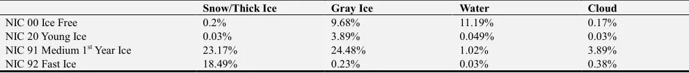
NIC provides a more comprehensive ice concentrations delineation. The MISI model is compared. Figure 11 shows the NIC catchment areas for various ice concentrations (a). All MISI pixels are queried within fast sea ice catchment (b);

within the medium 1st year ice catchment (c); and within the ice free catchment.

The percentage of each MISI pixel classification within each NIC catchment area are tabulated (Table 6). The table shows a possible delineation of thick ice and grey ice outside the medium 1st year ice catchment area.

Table 5. MISI Performance evaluation in IMS ice prediction using sensitivity and specificity tests.

MISI Ice Prediction

IMS Ice snow/thick ice snow/thick/gray ice water

T

ice (TP) = 1410 (40.98%) (TP) = 2419 (40.98%+29.33%) (FP) = 86 (2.5%)

E S

water (FN) = 26 (0.75%) (FN) = 345 (0.75%+9.27%) (TN) = 348 (10.11%)

T

sens = 1410/(1410+26) = 0.98 sens = 2419/(2419+345) = 0.87 spec=348/(348+86) = 0.80

Accuracy = 94.01% Accuracy = 86.52%

Figure 11. (a) NIC catchment areas. Spatial query of MISI pixels within (b) NIC CT92; (c) NIC CT91; (d) NIC CT00.

Table 6. Percentage of MISI classified pixels within NIC catchment areas.

Snow/Thick Ice Gray Ice Water Cloud

NIC 00 Ice Free 0.2% 9.68% 11.19% 0.17%

NIC 20 Young Ice 0.03% 3.89% 0.049% 0.03%

NIC 91 Medium 1st_{Year Ice} _23.17% _24.48% _1.02% _3.89%

NIC 92 Fast Ice 18.49% 0.23% 0.03% 0.38%

5. Conclusion

A dynamic threshold is an alternative to Bidirectional Reflectance Distribution Function (BRDF) correction which accounts for the biophysical, reflectance, and specular properties of a surface. In this study, a dynamic threshold based on lake ice detection method using an hourly threshold is developed. The threshold values are calculated on an hourly basis and applied to an ice detection algorithm through each iteration. The algorithm has been applied over Lake Michigan, one of five of the Great Lakes. Both fixed and dynamic thresholds have been compared. The resulting composite map using dynamic threshold yields significantly less unclassified pixels then the composite map using fixed threshold. A preliminary quantitative evaluation of the algorithm against IMS reveals good performance when delineating thick ice from water but lower performance when delineating gray ice from water. The use of a dynamic threshold may be used in constructing ice maps in applications that require higher temporal resolution. Future work proposed in this area

includes additional yearly test scenes of the same region in identical solar-view geometries to validate the robustness of the dynamic threshold followed by the development of additional dynamic threshold for other solar-view geometries, in the same region.

Acknowledgements

(10)

References

[1] Nazari, R., Khanbilvardi, R., and Cryosphere, N. C. 2011. “Fractional Ice mapping and monitoring for the future GOES-R Advanced Baseline Imager (ABI).” AGU Fall Meeting Abstracts. doi: 10.2011/AGUFM. C31A0595N.

[2] Nazari, R., and Khanbilvardi, R. 2011. “Application of dynamic threshold in sea and lake ice mapping and monitoring.”

International Journal of Hydrology Science and Technology. 1 (1/2): 37-46. doi: 10.1504/IJHST.2011.040739.

[3] Romanov, P., Gutman, G., and Csiszar, I. 2000. Automated monitoring of snow cover over North America with multispectral satellite data. J. Appl. Meteorol. 39 (11): 1866– 1880. doi: 10.1175/1520-0450 (2000) 039<1866:AMOSCO>2.0. CO; 2.

[4] Dorofy, P., Nazari, R., Romanov, P., and Key, J. 2016 “Development of a Mid-Infrared Sea and Lake Ice Index (MISI) Using the GOES Imager.” Remote Sens. 8 (12): 1015. doi: 10.3390/rs8121015.

[5] Liu, Y., Key, J., and Mahoney, R. 2016. “Sea and Freshwater ice concentration from VIIRS on Suomi NPP and the future JPSS satellites.” Remote Sens. 8 (6): 523. doi: 10.3390/rs8060523.

[6] Singh, P. Snow and glacier hydrology (37). Springer Science & Business Media. 2001.

[7] “Retrieval of surface albedo from space.” www2.hawaii.edu,

2017. Accessed 1 Feb 2017.

http://www2.hawaii.edu/~jmaurer/albedo/.

[8] Sandmeier, S. R., and Strahler, A. H. 2000. “BRDF laboratory measurements.” Remote Sensing Reviews. 18 (2-4): 481-502. doi: 10.1080/02757250009532398.

[9] Dumont, M., Brissaud, O., Picard, G., Schmitt, B., Gallet, J. C., and Arnaud, Y. 2010. “High-accuracy measurements of snow Bidirectional Reflectance Distribution Function at visible and NIR wavelengths–comparison with modelling results.”

Atmospheric Chemistry and Physics. 10 (5): 2507-2520. doi: 10.5194/acp-10-2507-2010.

[10] Gatebe, C. K., and King, M. D. 2016. “Airborne spectral BRDF of various surface types (ocean, vegetation, snow, desert, wetlands, cloud decks, smoke layers) for remote sensing applications.” Remote Sensing of Environment. 179 (15): 131-148. doi: 10.1016/j.rse.2016.03.029.

[11] Noguchi, K., Richter, A., Rozanov, V., Rozanov, A., Burrows, J. P., Irie, H. and Kita, K. 2014. “Effect of surface BRDF of various land cover types on geostationary observations of tropospheric NO2.” Atmospheric Measurement Techniques. 7

(10): 3497-3508. doi: 10.5194/amt-7-3497-2014.