www.mech-sci.net/6/245/2015/ doi:10.5194/ms-6-245-2015
© Author(s) 2015. CC Attribution 3.0 License.
Successive dynamic programming and subsequent
spline optimization for smooth time optimal robot
path tracking
M. Oberherber, H. Gattringer, and A. Müller
Institute of Robotics, Johannes Kepler University Linz, Altenbergerstr. 69, 4040 Linz, Austria
Correspondence to: M. Oberherber ([email protected])
Received: 28 May 2015 – Revised: 3 September 2015 – Accepted: 1 October 2015 – Published: 26 October 2015
Abstract. The time optimal path tracking for industrial robots regards the problem of generating trajectories that follow predefined end-effector (EE) paths in shortest time possible taking into account kinematic and dynamic constraints. The complicated tasks used in industrial applications lead to very long EE paths. At the same time smooth trajectories are mandatory in order to increase the service life.
The consideration of jerk and torque rate restrictions, necessary to achieve smooth trajectories, causes enor-mous numerical effort, and increases computation times. This is in particular due to the high number of optimiza-tion variables required for long geometric paths. In this paper we propose an approach where the path is split into segments. For each individual segment a smooth time optimal trajectory is determined and represented by a spline. The overall trajectory is then found by assembling these splines to the solution for the whole path. Further we will show that by using splines, the jerks are automatically bounded so that the jerk constraints do not have to be imposed in the optimization, which reduces the computational complexity. We present experimental results for a six-axis industrial robot. The proposed approach provides smooth time optimal trajectories for arbitrary long geometric paths in an efficient way.
1 Introduction
Highly automated production lines with efficient exploitation of the available resources become increasingly important for high wage countries to stay competitive. The utilization of present hardware plays a central role. This can be achieved by an intelligent path planning, using mathematical models of the mechanics to consider technical constraints in an opti-mization for the determination of optimal motions. It is an es-tablished approach to divide the problem into the geometric path planning using a scalar path parametersand optimiza-tion (Bobrow et al., 1985; Pfeiffer and Johanni, 1987). The path planning can for instance be done by combining lines and circles via clothoids. A popular and comfortable way is the definition of the path using polynomials or splines (Geu Flores and Kecskemethy, 2012; Gattringer et al., 2014). In Quang-Cuong (2014) a classification is proposed to divide optimization strategies deriving an optimal trajectory in the 2-D-phase space with coordinates (s,s) into three families:˙
1. Dynamic programming (DP): the phase space is divided into a discrete grid. Based on Bellman’s optimality prin-ciple (Bellman and Dreyfus, 1962) an optimal trajectory is derived on this grid (Shin and McKay, 1985).
2. Numerical integration: the optimal solution for the path parameter time evolution is obtained by integrating maximum and minimum accelerations and finding op-timal switching points for this acceleration and de-celeration periods in the phase plane (Bobrow et al., 1985; Pfeiffer and Johanni, 1987). Geu Flores and Kecskemethy (2012) used this method to solve the so-called generalized waiter motion problem.
246 M. Oberherber: Smooth time optimal robot path tracking The tasks to be performed in industrial applications often
contain long paths with rough as well as fine contours. Fur-thermore, the movement should be precise in order to com-ply with required accuracies on the one hand, and the motor torques should be smooth in order to avoid vibrations and to protect the hardware. Short optimization times are also cru-cial in order that the saving in execution time is not annihi-lated by increased calculation times.
To overcome these demands, one may start to optimize the whole path using one approach mentioned above consider-ing kinematic (joint velocity and acceleration) and dynamic (torque) constraints. Smooth trajectories can be achieved by taking jerk or torque rate restrictions into account. In Con-stantinescu and Croft (2000) and Oberherber et al. (2014) methods to consider them in phase space are presented, while Debrouwere et al. (2013) proposes a sequential con-vex scheme to solve a nonlinear program. However, for stan-dard six axis industrial robots and long geometric paths the calculation effort is enormous due to the high number of opti-mization variables and restrictions. This is also caused by the fine discretization, required for a detailed implementation of fine structures of the geometric path. A non-equidistant cretization, where only certain regions of the path are dis-cretized finely, would be a first choice to reduce the size of the problem. But, if the path is very long and contains many finely discretized regions, this approach is not feasible. An-other way to reduce the number of optimization variables is a decomposition of the path into segments, performing the optimization for the segments and assembling the solutions to the whole optimal trajectory. In order to achieve a con-tinuous trajectory, terminal conditions have to be defined at the intersection points and regarded in the optimization. We use a DP approach to calculate optimal trajectories for each segment and subsequently for the entire path. For this task we consider restrictions of path velocity, joint velocity and acceleration and also torque limits. Neglecting the jerk re-strictions is reflected in a bang-bang behavior of the motor torques.
To obtain smooth robot movements in short optimization times, we approximate the solution provided by the DP ap-proach for each segment of the path with a spline. Subse-quently, this approximation is used as initial guess for the optimization of the spline using an active-set solver (No-cedal and Wright, 2006), considering the same restrictions as before. The degree of the splines and the number of con-trol points determine the smoothness of the solution. Since the initial state is near to the global optimum, the calculation times remain low.
As the initial state for the spline optimization is derived by a DP approach, the first part can be assigned to category one. A categorization of the spline optimization is not really possible, since we use an active set solver to optimize the non-convex problem.
The paper is organized as follows: in Sect. 2 the geometric path, describing the task the robot should perform, is defined.
Section 3 treats the time optimal path planning problem in the parameter space in a general way, Sect. 4 introduces our solution strategy. Section 5 addresses the used optimization based on DP in detail. An approach to attain smooth trajec-tories with short calculation times is introduced in Sect. 6. Experimental results, realized on a Stäubli RX130L – a six-axis industrial robot, are presented in Sect. 7.
In this paper we use the abbreviation( )˙ = d
dt for the time derivative of a quantity. The derivative with respect to the path parameter is denoted with ( )0= d
ds. Bold lower case letters characterize vectors, while capital letters are used for matrices with the exception of commonly used notations in mechanics. The euclidean norm of the vectorx is denoted withkxk.
2 Geometric path planning
The aim of path planning is the definition of the robot’s task. There are several methods to define such a geometric path, like polynomials, combination of lines, circles and clothoids (Müller et al., 2007) or splines (Bobrow, 1988; Gattringer et al., 2014). The latter provide a comfortable way to define the robots motion whether in joint coordinatesqor in Cartesian coordinateszE. To consider obstacles in the workspace, it is
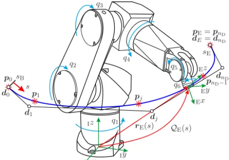
common to define the geometric path in the Cartesian space as shown in Fig. 1.
A three-dimensional spline curve, describing the end-effector position can be written as
rE(s)= nD
X
l=1
dlNld(s), (1)
with the scalar path parameters= [sB, sE](sB– begin of the
path,sE– end of the path), and thenDcontrol pointsdl defin-ing the shape of the curve. These control points can either be defined directly or can be determined using interpolation pointspl as shown in Gattringer et al. (2014).Nld(s) denote the B-spline basis functions of degreed. There are different ways to define this basis functions as local or global support functions. For details we refer to De Boor (1978) and Piegl and Tiller (1995). Unit Quaternions Q=e0,eTT (scalar
parte0and vector part e) are used for the definition of the
end-effector orientation QE. The evolution of the separate
coordinatese0,ex,ey andezalong the path is again defined via splines with a subsequent normalization. The angular velocity of the end-effector, represented in the end-effector frame, can be calculated toEωE=2 [e0e˙−eee˙−ee˙0].
3 Time optimal path tracking
3.1 Problem description
M. Oberherber: Smooth time optimal robot path tracking 247
q1 q2
q3
q4
q5
q6
d0
d1 d
j
dnD−1
dE=dnD
p0
p1 pj
pnD−1
pE=pnD
Ix Iy Iz
Ex Ey Ez
s sB
sE
rE(s) QE(s)
Figure 1.Six-axis industrial robot with geometric path.
s(t). This is accomplished with an optimization considering technical constraints like motor-torque, velocity and acceler-ation restrictions. The general formulacceler-ation of the path track-ing problem is given by
min tE∈R+,τ(·)
tE
Z
0
k1+k2τTτ
dt, (2)
whereinτ denotes the vector of motor torques as a function of time. With the coefficientsk1andk2a weighting between
time and energy optimality can be achieved. Basically we are able to handle this general case, but in this paper we concentrate on time optimal solutions, therefore the factors k1=1 andk2=0 are used and the torques vanish from the
cost function. The cycle time tE represents the solution of
the optimization and is consequently an unknown quantity. A change of the integration variable fromttosleads to
tE= tE
Z
0
1 dt= sE
Z
sB 1 ˙
s(s)ds (3)
and the optimization problem can be written as
min
˙ s(·)
sE
Z
sB 1 ˙
s(s)ds. (4)
3.2 Technical constraints 3.2.1 Process constraints
For the trajectory optimization several technical constraints should be considered. The first one concerns the end-effector velocity vE=
drE
dt
, which is a process related restriction.
Such constraints can be found in grinding or welding opera-tions. By using the chain rule
dx dt =
dx ds
ds dt =
dx dss˙=x
0˙
s, (5)
the path velocity follows as
vE=
drE
ds ds dt
=r0E(s)
s˙ (6)
in the parameter range.
3.2.2 Manipulator constraints
Restrictions imposed by the used hardware concern the mo-tor mo-torque, joint velocity, and joint acceleration. In Sect. 2 the path is determined in Cartesian coordinates whereas these restrictions are defined in joint coordinates. Since the end-effector coordinates are calculated with the forward kinemat-icszE= [rT
EQTE]T =f(q) for desired joint positions, the
in-verse kinematicsq(s)=f−1(zE(s)) provides the joint angles for desired end-effector coordinates. There are different ways to solve this locally, but not globally unique problem. We use a numerical approach based on the relation
vE
ωE
=J(q)q˙ , (7)
with the end-effector velocitiesvE,ωErepresented in the
in-ertial frame and the Jacobian
J= ∂vE
∂q˙ ∂ωE
∂q˙
!
. (8)
With the chain rule Eq. (5), the joint velocity and acceler-ation follow as
˙
q=dq dss˙=q
0s˙ (9)
¨
q=q00s˙2+1 2q
0
(s˙2)0. (10)
The end-effector prime quantities are calculated, using
z0E(s)=
h
r0E(s)T
,(ωE(s))T iT
,
z00E(s)=
h
r00E(s
)T, ω0E(s)TiT
and the Jacobian J
q0=J−1z0E (11)
q00=J−1
z00E−J0q0
. (12)
In order to formulate the torque restrictions, a dynamic model of the robot is necessary. It is derived with the help of the Pro-jection Equation (Bremer, 2008) resulting in the Equations of Motion (EoM)
248 M. Oberherber: Smooth time optimal robot path tracking Coriolis-, gravitational-, centrifugal- and friction forces are
contained ing. The motor torques are represented byτ. As well as the velocity and acceleration restrictions Eqs. (6), (11), (12), also the torque restrictions are required in terms of the path parameter. There exist different ways to express the EoM in terms of the path parameter as those proposed in Johanni (1988) and Geu Flores and Kecskemethy (2012). An analytical formulation is shown in Gattringer et al. (2014), where the parametrized EoM are written as
τ =a(s)(s˙2)0+b(s)s˙2+c(s)+dv(s)s.˙ (14)
The coefficientsa,b, c anddvof the parametrized EoM
fol-low directly by rewriting and parametrizing the Projection Equation.
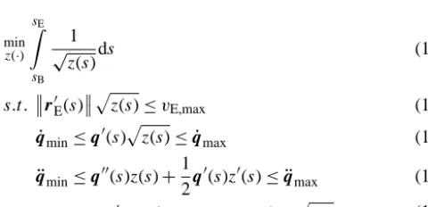
By introducing the variablez= ˙s2the optimization prob-lem in parameter space follows as
min z(·)
sE
Z
sB 1 √
z(s)ds (15)
s.t. r0E(s)
p
z(s)≤vE,max (16)
˙
qmin≤q0(s)pz(s)≤ ˙qmax (17) ¨
qmin≤q00(s)z(s)+1 2q
0(s)z0(s)≤ ¨q
max (18)
τmin≤a(s)z0(s)+b(s)z(s)+c(s)+dv(s)
p
z(s)≤τmax. (19)
The values for the motor torque restrictions τmin, τmax
and joint velocity restrictions q˙min,q˙maxcan be taken from the data sheets of the motors respectively gears. Generally the lower limits are equal to the negative values of the upper limits: τmin= −τmaxandq˙min= − ˙qmax. The same applies
to the acceleration restrictionsq¨min= − ¨qmax, which are usu-ally defined in the joint controllers. Depending on the process to be performed, the path velocity limit vE,max is set to the
optimal working speed.
The better the robot model matches the real system, the better the limits can be exploited. Primarily parameters that are necessary to simulate the kinematics, like link lengths or distances between axis can be taken from CAD – data. The parameters for the dynamic model – masses, centers of grav-ity or inertia tensors can usually only be estimated with CAD models. For a good match of the derived robot model with the real system, a parameter identification as shown in Neubauer et al. (2014) and Swevers et al. (1996) is indispensable.
4 General solution strategy
The requirements of smooth time optimal trajectories for long geometric paths and short computation times were dis-cussed in Sect. 1 as well as our idea to overcome this chal-lenge. A reduction of optimization variables for a particular optimization is achieved by dividing the path into sections and performing the optimization for these segments. To get
z
s sB=s1,b
zmax
zopt,1
zopt,2
zpr,1
zpr,2
so,1
so,2 sp,1
sp,2 s2,b
s1,e
s2,e
z(s1) z′(s1)
z(s2) z′(s2)
Figure 2. Solution strategy: successive dynamic programming
(SDP).
smooth trajectories in acceptable calculation times, we define the evolution ofz(s) in the “phase space”s×zas a smooth spline curve and optimize its shape with an active-set solver. For this kind of problem a suitable initial guessz0(s) is
cru-cial but is not always easy to define. In Verscheure et al. (2009) a parabola is used. This approach works reasonably well for zero velocity at the begin and end of the path, but is not guaranteed to work in the general case of desired start and end velocities. The division of the path into segments makes their consideration mandatory to achieve a continuous over-all trajectory. For that purpose we propose an elegant way to derive the initial states by using a DP approach consider-ing the terminal conditions and approximate its solution with a spline curve. Since the DP approach provides the global optimum, it yields an excellent approximation. However, the discretization for this algorithm can be chosen coarse in or-der to save computation time, since it only provides the initial states for a further optimization of the spline curve.
The piecewise optimization procedure is sketched in Fig. 2. It starts with the definition of an optimizationsoand
a prediction horizonsp. FromsBtoso,1+sp,1=s1,ethe
op-timization is performed and provides an optimal trend, that is split intozopt,1 andzpr,1. Along the optimization horizon
the optimal trajectory is stored and used as a part of the op-timal trajectory of the whole path. The prediction horizon is necessary to determine the terminal conditions. At the end of the optimization horizonz(s1) andz0(s1) are stored as
termi-nal conditions. Afterwards the horizons are shifted forward byso,1 and the next optimization starts ats2,b and leads to
s2,b+so,2+sp,2=s2,e under consideration of z(s1), z0(s1).
This procedure is repeated till the end of the path is reached. In further consequence we will call the sequential execution of the algorithm successive dynamic programming (SDP).
z z′
zL
zmax(si)
zmin(si)
z′.. q+1
z..′ q+2
zτ′+ 1
z′ τ2+
z′.. q−1
z′..q− 2
z′ τ1−
z′τ− 2
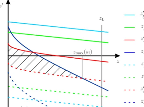
Figure 3.Graphical illustration of technical restrictions in thez×z0 plane.
horizon effects unnecessary deceleration phases. A general choice can not be proposed, rather they have to be chosen problem dependent.
5 Dynamic programming approach to determine an
initial solution
5.1 Graphical illustration of restrictions
For a fix point si on the path the restrictions in Eqs. (16)– (19) can be graphically illustrated in thez×z0plane. This is exemplary shown in Fig. 3 fork=2 degrees of freedom and with the assumption that the lower restrictions are equal to the negative upper restriction values.
The velocity restrictions can be squared and combined to
zL=min "
˙ qk,2max
q02 k
,v
2 E, max
r0E
2
#
(20)
representing a vertical line in thez×z0plane. For each joint the acceleration limits follow to
z0¨ qk±=
2 ± ¨qk,max−qk00z
qk0 (21)
and thus to linear functions in the z×z0 plane. Due to the consideration of viscous friction (coefficientdv) each joints
torque restriction follows to
z0 τk±=
bk ak
z+ck ak
+dv,k ak
√
z±τk,max ak
(22)
and thus to nonlinear functions in thez×z0plane.
The set of curves provide a feasible region (shaded in Fig. 3) for the states. Significant points are given by the minimum and maximum feasible values of z, denoted with
zmin(si) andzmax(si). In Fig. 3zmin(si) is equal to zero. Since a numerical method is used to derive the feasible region it is also possible to consider valueszmin(si)>0, as they occur for example at the so-called waiter motion problem in Geu Flores and Kecskemethy (2012).zmax(si) can either be given by the intersection point of the lowest upper with the highest lower restriction or can concur with the velocity restriction zL. Within the rangez=zmin. . .zmax(si) the feasible region defines the minimumz0(z) and maximumz0(z) allowed gra-dients.
5.2 Discretizing the problem
The DP approach is based on Bellman’s optimality princi-ple. “[...] An optimal policy has the property that whatever the initial state and the initial decision are, the remaining de-cisions must constitute an optimal policy with regard to the state resulting from the first decision (Bellman and Dreyfus, 1962) [...]”.
With a process running backwards, these decisions can be picked up and optimized with respect to a desired optimal-ity. For that purpose the first step is to discretize the whole path inton segments s=sB. . .si. . .sE with a discretization
step size1s=sE−sB
n andi=0. . .n. Then the optimization horizonsowithnodiscrete points and prediction horizonsp
withnp discrete points are chosen as integral multiples of
1s. In the following only one segments=sb. . .seis
consid-ered, where the start point is denoted withsband the endpoint
withse. Afterwards we evaluate the minimumzmin(si) and maximum admissible valueszmax(si) at all discrete points as shown in Fig. 3 resulting in the limiting curveszmin(s) and
zmax(s), that provide the base of operations. Furtherzis
dis-cretized with the step size1z=zmax(si)−zmin(si)
m intompieces in the rangez=zmin(si). . .zmin(si)+j 1z. . .zmax(si) withj= 0. . .m. The treatment of the path sections leads to a discrete (no+np)×mgrid instead of an×mgrid (no+np< n) in
the phase plane. Within this grid also the cost functional from Eq. (15) has to be discretized to
W= ne
X
i=nb 1s √
zi
(23)
withnb=sb/1sandne=se/1s.
5.3 Successive dynamic programming
The backwards running process starts at the paths end by ini-tializing the cost functionW. Starting from a desired end ve-locity represented byze the gradients to all velocity points
ze−1,j on the path pointse−1are calculated with
z0e−1,j=ze−1,j−ze
1s . (24)
250 M. Oberherber: Smooth time optimal robot path tracking
z zj
z′
z′ j 0
z′ j
z′(z)
z′(z) zmax
Figure 4.Feasible region in thez×z0plane with maxz0j and min z0jatzj.
by Fig. 4. The cost function is initialized withWe−1,j=√1sz j at points with valid gradients (green solid in Fig. 5) and with We−1,j→ ∞ for points with invalid gradients (green dashed). With the cost function on hand the proceeding can be continued for the path points se−2. . .sb. At these points
the cost function has to be considered in the calculation of the optimal gradients. This is accomplished by determin-ing the minimum and maximum allowed gradientsz0i,j and z0i,j using Fig. 4 of the actual pointzi,j and calculating the covered range [zi,j, zi,j] at the following path point si+1.
Within this range along the zaxis the location of the cost functions minimum z∗i,j has to be found. A popular proce-dure is a minimum search based on the golden ratio. How-ever, we take advantage of its special shape for purely time optimal trajectories W=1s√
z . A closer examination shows that the minimum is located at the highest value ofzwhich leads to a feasible value different to∞. This step is reflected in a strongly reduced computation time. With z∗i,j the
op-timal gradient follows to z0i,j=z
∗
i,j−zi,j
1s and the cost func-tion is adapted toWi,j =Wi+1,j+√1sz
i,j or Wi,j→ ∞if it is out of range. The whole procedure has to be executed for every discrete point at the remainingne−nb−2×mgrid.
After completion of the optimal gradient determination, the optimal evolution of z(s) can be calculated iteratively with zopt,i+1=zopt,i+zi,j0 1s(blue in Fig. 5), starting with a de-sired start valuezopt(sb)=zband a valid gradientz0(sb)=zb0
provided by the terminal conditions.
6 Spline based smoothing of the initial solution
6.1 Local spline approximation
The solution provided by the DP approach in Sect. 5 leads to a bang-bang – behavior in the motor torques, resulting in heavy stress for the actuators and the mechanics. In Ober-herber et al. (2014) an approach is proposed, that considers torque derivative and joint jerk restrictions in the optimiza-tion. This extension of the DP algorithm results in long cal-culation times and is thus not feasible for long paths. For this reason, we propose a different way in this paper to obtain
z z
zmax
z∗
i,j zi,j z′
i,j z′
i,j
z
′i,j
zi,j zi,j
sb sb+1 si se−1 se Wopt ∞ W
ze
zb
ze′
z′b
zopt
0 0
Figure 5.Dynamic programming algorithm.
z
s
sb se
zmax zopt
ˆ
z0
ˆ
zopt
ˆ
d0
ˆ
d
Figure 6.Spline approximation and optimal solution.
smooth trajectories. We approximate the optimal evolution of zopt(s) derived by the dynamic programming algorithm,
with a spline curve.
In a first step the trend ofz(s) is expressed as a spline
ˆ z0(s)=
ˆ nD
X
l=1
Nld(s)dˆ0,l (25)
whosenˆDcontrol pointsdˆ0follow from a least squares
ap-proximation
min
ˆ
d0∈RnˆD
ne
X
i=nb
zˆ0(si)−zopt(si)
2
(26)
minimizing the error between optimal and approximated trend at the discrete pointss=sb, sb+1s. . .si, . . .se of the
DP algorithm. The splinezˆ0(s) is discretized to the originally
demanded fine discretization1ˆs=sE−sB ˆ
n withn > n.ˆ
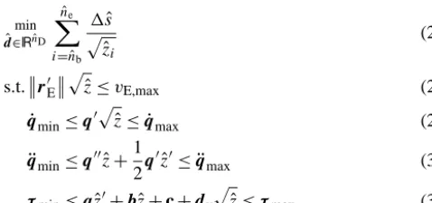
6.2 Ensuring consistency 6.2.1 Optimization problem
in order to satisfy the restrictions at all discrete points. The optimization problem that has to be solved to fulfill the re-strictions is
min
ˆ
d∈RnˆD
ˆ ne
X
i= ˆnb 1sˆ
p
ˆ zi
(27)
s.t.r0E
p
ˆ
z≤vE,max (28)
˙
qmin≤q0pzˆ≤ ˙qmax (29) ¨
qmin≤q00zˆ+1 2q
0ˆ
z0≤ ¨qmax (30)
τmin≤azˆ0+bzˆ+c+dv p
ˆ
z≤τmax (31)
withnˆb=sb/1sˆ andnˆe=se/1s. Figure 6 shows the SDPˆ
solution zopt and the approximation zˆ0(s) with the control
points d0 used as initial states for the optimization. The
smooth time optimal trajectoryzˆopt(s) follows from the
opti-mal control pointsdˆ provided by the optimization Eqs. (27)– (31).
6.2.2 Gradients
For a fine discretization, the restriction check at every dis-crete point is computationally expensive. A significant cal-culation time reduction can be achieved by providing analyt-ical expressions for the gradients of the cost functional and restrictions with respect to the optimization variables. There are actually software tools to compute gradient and Hessians using automatic differentiation. Nevertheless, as the restric-tions and the objective are given as analytical funcrestric-tions of the optimization variables, the gradients can easily be calculated analytically. By inserting the spline zˆopt(s)=Pnlˆ=D1N
d l(s)dˆl into the discrete cost functional
W = ˆ ne
X
i= ˆnb 1sˆ
p
ˆ zopt,i
, (32)
its gradient regarding the optimization variablesdˆlfollows to
∂W
∂dˆl =
ˆ ne
X
i= ˆnb −1
21sNˆ d l,i
ˆ zopt,i
3 2
. (33)
Inserting the spline and its derivative with respect to the path parameterzˆ0opt(s)=PnˆD
l=1Nld 0
(s)dˆl into the restrictions, their gradients regarding the optimization variablesdˆlfollow to
∂vE
∂dˆl = 1
2
r0E
Nld
p
ˆ zopt
(34)
∂q˙ ∂dˆl
= 1 2q
0 N d l
p
ˆ zopt
(35)
∂q¨ ∂dˆl
= q00Nld+1 2q
0
Nld0 (36)
∂τ
∂dˆl
= aNld0+bNld+1 2dv
Nld
p
ˆ zopt
. (37)
6.2.3 Terminal conditions
To achieve a continuous trajectory a consideration of the ter-minal conditions for the spline optimization is necessary, as with the DP algorithm. For this purpose the first two control points have to be calculated separately. The first control point is defined by the terminal condition forz(sb)
d1=z(sb), (38)
while the second control point follows to
d2=z0(sb)−d1
N1d0(sb)
N2d0(sb)
(39)
for a transition gradient z0(sb) and the derivatives of the
first two basis functions N1d0 and N2d0 with respect to the path parameter If also transition conditionsz(se)=ze and
z0(se)=z0eat the end of the path are required, the same
pro-cedure also works for the last and second last control point. The definition ofz(s) as spline entails a further advantage namely an easy way to achieve a smooth start and stop. Jerky accelerations at the beginning and decelerations at the end of the path lead to end-effector vibrations which are problemat-ical especial for elastic systems since they need a long time to settle to the desired endpoint. The definition ofz0(sb)=0
leads to a smooth start whilez0(se)=0 provides a smooth
stop.
7 Results
The experiments are realized with a Stäbli RX130L, a six-axis industrial robot. It is controlled by a Bernecker und Rainer system with PD controller and torque feed forward control for each joint. We use a spline curve of degreed=4 in form of our institute logo (a robin), shown in Fig. 7, as geometric path. It is aboutl≈7.8 m long and is discretized intonˆ=2000 pieces to represent even the fine contours. The end-effector orientation is held constant equal to the initial orientation, so that an observer directly faces the robots end-point.
For the calculation of the initial solution for the spline op-timization with the SDP algorithm the velocity discretization amountsm=300, while the path is discretized inton=250 in the rangesB=0. . .sE=1. As horizonsso=0.2 (50
seg-ments) andsp=0.08 (20 segments) are defined which lead
to a subdivision of the total path into five segments.
Figure 8 shows the phase planes×zwith the liming curve zmax, the optimal evolution zopt provided by the SDP
ap-proach and the smooth optimal trendzˆopt. This spline curve
of degree d=4 contains nˆD=40 control points for each
path segment.
252 M. Oberherber: Smooth time optimal robot path tracking
z
in
m
yin m xin m
s sB sE
1.2
0.4
−1 −0.4 −0.2
0
0
0 0.2
0.5 0.5
−0.5
0.6
0.8
1
1 1
Figure 7.Geometric path – logo of the Institute of Robotics at the
JKU Linz.
ˆ
zopt zopt
zmax
z
pathparameters
0 0.2 0.4 0.6 0.8 1
0
0.05
0.1
0.15
0.2
0.25
0.3
0.35
0.4
Figure 8. Limiting curve and optimal evolution of the SDP
ap-proach and for the smooth solution.
a smooth start and stop, where the torques run into the static torques. The difference becomes clearer by looking at the torque rates in Fig. 10 and the joint jerks in Fig. 11. Fig-ure 10 shows, that the torque rates of the discontinuous tra-jectory are approximately ten times higher then the torque rates of the smooth solution withnˆD=40 control points for
each section.
The smoothness of the trajectory contrasts with an increas-ing execution time from tE≈3.72 s for the bang bang
so-lution to tE≈4.02 s for the smooth solution with nˆD=40
control points for each section. This smooth trajectory was successfully implemented in simulations as well as on the real system, a video clip of the implementation is available on https://youtu.be/c5jllkLE4oU. A reduction of the number of control points tonˆD=25 leads to a smoother solution, but
increases the execution time totE≈4.22 s. Figure 11 shows
the joint jerks for the different cases. One can see, that the
timetin s
τ
τmax τ6
τ5 τ4 τ3 τ2 τ1 τ
τmax
0 1 2 3 4
0 0.5 1 1.5 2 2.5 3 3.5
−1 −0.5
0
0.5
1
−1 −0.5
0
0.5
1
Figure 9.Motor torques, above: torque trends for the SDP solution,
below: torque trends for the smooth solution.
timetin s
. τin
N
m
/s
. τ6
. τ5
. τ4
. τ3
. τ2
. τ1
. τin
N
m
/s
0 1 2 3 4
0 1 2 3
×104
−500
0 500 1000
−1 −0.5
0
0.5
1
Figure 10.Motor torque rates, above: torque rate trends for the
SDP solution, below: torque rate trends for the smooth solution.
reduction of the number of control points increases the exe-cution time but reduces the joint jerks.
For validation purposes we implemented an optimization with hard jerk constraints...qmax=3000rad
s3 , considered in the spline optimization. This optimization converges only for a low number of control points up tonˆD=25. The calculation
time rises totCPU≈65 s, while the execution timetE≈4.13 s
is nearly the same as without jerk restrictions.
Finally we tried to calculate a time optimal trajectory for the whole path in one go, withnˆD=100 control points. For
... qin
ra
d/
s
3
timetin s
... qin
ra
d/
s
3
... q6 ... q5 ... q4 ... q3 ... q2 ... q1 ... qin
ra
d/
s
3
0 1 2 3 4
0 1 2 3 4
0 1 2 3
×104
−4000 −20000
2000 4000
−5000
0 5000
−5
0 5
Figure 11. Joint jerks, above: trend of joint jerks for the SDP
approach, middle: trend of joint jerks for a smooth solution with ˆ
nD=40 control points for each section, below: trend of joint jerks
for a smooth solution withnˆD=25 control points for each section.
the whole path, and inspired by Verscheure et al. (2009), a parabola trend of the control points. For that purpose the lo-cations of the control pointsdˆ are defined as
ˆ
dk+1= −min (zmax)
4k − ˆnD+k+1
ˆ nD−1
2 , (40)
withk=1, . . .,nˆDanddˆ0=0. The factor min(zmax) ensures,
that no velocity restriction is violated by the initial guess. Both approaches require a coarse discretization of the path (nˆ=1250) to achieve a convergence of the spline optimiza-tion. Despite the coarse discretization, the calculation times increase clearly. The slightly smaller execution timestEcan
be attributed to the coarser discretization.
The results of the different methods are listed in Table 1. In this table, SO is the abbreviation for spline optimization and g indicates the usage of analytical gradients. Jerk suggests the consideration of hard joint jerk restrictions in the spline optimization. The last two lines of Table 1 show the results for the optimization in one go with the DP and parabola ap-proach for the initial guess.
The spline optimization was done with the active-set algo-rithm of the Matlab optimizer fmincon. With the timetCPU
we indicate the computation time on a standard PC with a CPU clock of 2.83 GHz. The results in Table 1, clearly indi-cate the improvements of the presented approach compared to an approach with jerk constraints. Nevertheless, the calcu-lation times are significantly higher compared to the execu-tion times. An improvement could for example be achieved by implementing the optimization not in MATLAB, but in a C-based optimization toolbox.
Table 1.Trajectory execution timestEand calculation timestCPU
for the different methods.
Method tCPU tE nˆD nˆ
(s)
SDP 5 3.72 – 2000
SDP and SO 120 4.02 40 2000 SDP and SO and g 25 4.02 40 2000 SDP and SO and g 20 4.22 25 2000 SDP and SO and g and jerk 65 4.13 25 2000 DP and SO and g 58 4.01 100 1250 parabola and SO and g 101 4.01 100 1250
8 Conclusions
This paper presents an approach to derive smooth time opti-mal trajectories for arbitrary long geometric paths. The main idea is to split the path into sections, to calculate optimal trajectories using terminal conditions, and to assemble the solutions for the individual segments. To achieve smooth tra-jectories in acceptable calculation times we propose a spline optimization in the phase space. The problem of convenient initial states for the optimization is solved with a DP ap-proach in which terminal conditions can be considered in an easy way. With the spline optimization it is also simple to achieve a smooth start and stop of the robot. The presented approach may be interesting for robot manufacturers which already have algorithms for the path tracking problem and want to extend them to achieve smooth trajectories. Exper-iments to show the proper functionality of the method are realized on a six-axis industrial robot. An extension of the algorithm to consider jerk and torque rate restrictions in the optimization will be part of future work.
Acknowledgements. This work has been supported by the
Austrian COMET-K2 program of the Linz Center of Mechatronics (LCM), and was funded by the Austrian federal government and the federal state of Upper Austria.
Edited by: M. Hofbaur
Reviewed by: two anonymous referees
References
Ardeshiri, T., Norlöf, M., Löfberg, J., and Hansson, A.: Convex op-timization approach for time optimal path tracking of robots with speed dependent constraints, in: Proceedings of the 18th IFAC Congress, Milano, Italy, 28 August–2 September 2011, 14648– 14653, 2011.
Bellman, R. E. and Dreyfus, S. E.: Applied Dynamic Programming, Princeton University Press, Princeton, New Jersey, USA, 1962. Bobrow, J. E.: Optimal Robot Path Planning Using the
254 M. Oberherber: Smooth time optimal robot path tracking Bobrow, J. E., Dubowsky, S., and Gibson, J. S.: Time-optimal
con-trol of robotic manipulators along specified paths, Int. J. Robot. Res., 4, 3–17, 1985.
Bremer, H.: Elastic Multibody Dynamics: A Direct Ritz Approach, Springer Netherlands, Dordrecht, Netherlands, 2008.
Constantinescu, D. and Croft, E. A.: Smooth and time-optimal trajectory planning for industrial manipulators along specified paths, J. Robot. Syst., 17, 233–249, 2000.
De Boor, C.: A practical guide to splines, Springer Verlag New York, New York, USA, 1978.
Debrouwere, F., Van Loock, W., Pipeleers, G., Tran Dinh, Q., Diehl, M., De Schutter, J., and Severs, J.: Time-Optimal Path Follow-ing for Robots with Trajectory Jerk Constraints usFollow-ing Sequential Quadratic Programming, in: Proceedings of IEEE ICRA 2013, 6–10 May 2013, Karlsruhe, Germany, 1916–1921, 2013. Gattringer, H., Oberherber, M., and Springer, K.: Extending
con-tinuous path trajectories to point-to-point trajectories by varying intermediate points, International Journal of Mechanics and Con-trol, 15, 35–43, 2014.
Geu Flores, F. and Kecskemethy, A.: Time-Optimal Path Planning Along Specified Trajectories, in: Multibody System Dynamics, Robotics and Control, edited by: Gattringer, H. and Gerstmayr, J., Springer Vienna, Wien, Austria, 1–16, 2012.
Johanni, R.: Optimale Bahnplanung bei Industrierobotern, VDI Ver-lag, Düsseldorf, Germany, 1988.
Müller, B., Deutscher, J., and Grodde, S.: Continuous Curvature Trajectory Design and Feedforward Control of Parking a Car, IEEE T. Contr. Syst. T., 15, 541–553, 2007.
Neubauer, M., Gattringer, H., and Bremer, H.: A persistent method for parameter identification of a seven-axes manipulator, Robot-ica, 1–14, 2014.
Nocedal, J. and Wright, S. J.: Numerical Optimization, 2nd Edn., Springer-Verlag New York, New York, USA, 2006.
Oberherber, M., Gattriger, H., and Springer, K.: Time Optimal Path Planning for Industrial Robots: A Dynamic Programming Ap-proach Considering Torque Derivative and Jerk Constraints, in: Proceedings in Applied Mathematics and Mechanics, 14, 75–76, 2014.
Pfeiffer, F. and Johanni, R.: A Concept for Manipulator Trajectory Planning, IEEE Journal of Robotics and Automation, 3, 115– 123, 1987.
Piegl, L. A. and Tiller, W.: The NURBS Book, 2, Springer-Verlag Berlin Heidelberg, Berlin, Germany, 1995.
Quang-Cuong, P.: A General, Fast, and Robust Implementation of the Time-Optimal Path Parameterization Algorithm, IEEE T. Robot., 30, 1533–1540, 2014.
Shin, K. and McKay, N.: Minimum-Time Control of Robotic Ma-nipulators with Geometric Path Constraints, IEEE T. Automat. Control, 30, 531–541, 1985.
Swevers, J., Ganseman, C., De Schutter, J., and Van Brussel, H.: Experimental robot identification using optimised periodic tra-jectories, Mech. Syst. Signal Pr., 10, 561–577, 1996.