A framework for measuring sharpness in natural images captured by digital cameras based on reference image and local areas

(1)

R E S E A R C H

Open Access

A framework for measuring sharpness in natural

images captured by digital cameras based on

reference image and local areas

Mikko Nuutinen

1*

, Olli Orenius

2

, Timo Säämänen

2

and Pirkko Oittinen

1

Abstract

Image quality is a vital criterion that guides the technical development of digital cameras. Traditionally, the image quality of digital cameras has been measured using test-targets and/or subjective tests. Subjective tests should be performed using natural images. It is difficult to establish the relationship between the results of artificial test targets and subjective data, however, because of the different test image types. We propose a framework for objective image quality metrics applied to natural images captured by digital cameras. The framework uses reference images captured by a high-quality reference camera to find image areas with appropriate structural energy for the quality attribute. In this study, the framework was set to measure sharpness. Based on the results, the mean performance for predicting subjective sharpness was clearly higher than that of the state-of-the-art algorithm and test-target sharpness metrics.

Keywords:image quality, reduced-reference metric, no-reference metric, test-target metric, camera phone, bench-marking, subjective sharpness

1. Introduction

Image quality can be measured using objective or subjec-tive methods. Different imaging applications require dif-ferent methods and metrics. Objective methods for characterizing the performance of digital cameras can be based on test-targets or algorithms. For a test-target metric, a target with known physical properties is cap-tured, and the reproduction is measured. Test-target measurements are tedious and require a controlled laboratory environment. Compared to a real scene, test-target views are easy to interpret and process as desired. Subjective tests, however, cannot utilize captured test-target images. Subjective tests for consumer cameras should be performed using natural-scene views captured under typical photographic conditions. Only natural scenes can show the naturalness and usefulness of images captured by a camera.

Algorithmic methods can facilitate natural-scene pic-ture assessment, and the same image files can be used for

both subjective and objective measurements. The algo-rithmic methods can be classified into no-reference (NR), reduced-reference (RR), and full-reference (FR) methods. This classification is related to reference images’ avail-ability and use. An NR metric does not need a reference image, an RR metric needs some information about a reference, and an FR metric needs a pixel-wise reference image.“Pixel-wise”means that the corresponding pixels in two images are found at the same pixel coordinate locations. This is not the case when characterizing cam-eras, e.g., for benchmarking purposes.

Objective image-quality research aims to develop meth-ods that predict the subjective quality experience. The FR methods are fairly close to achieving this goal [1]. There are different approaches to the FR methods. One is based on modeling the human visual system [2], and another is based on the structural similarity (SSIM) between images [3]. In addition, natural image statistic (NSS) metrics are promising [4]. The SSIM metric is simple and has many variations [5-8]. Recently, eye-tracking and salience algo-rithms have been integrated into FR methods [9-12]. These algorithms weight the attractive areas of an image when the spatial values of the quality metrics are pooled

* Correspondence: [email protected] 1

Department of Media Technology, Aalto University School of Science, P.O. Box 15500, FI00076 Aalto, Finland

Full list of author information is available at the end of the article

(2)

into a single quality number. Learning-based models are another new direction. Examples include Moorthy and Bovik’s [13] learned-support vector machine, Eerola’s [14] learned-Bayesian network, and Cui and Allen’s [15] learned neural networks for estimating image quality.

An FR metric is often general. Its output is a single number (e.g., a mean of a spatial distortion map) that pro-vides an overall quality estimation. If the image-quality space is multi-dimensional, as with digital cameras, a sin-gle number or distortion map does not explain the quality [16]. Image-quality evaluation can be seen as a hierarchical model. The model includes higher- and lower-level attri-butes. The higher-level attributes are more subjective. Personal preferences affect their values more than those of the lower-level attributes. For example, naturalness and clarity are higher-level attributes for a consumer digital camera. Graininess, brightness, sharpness, and contrast are lower-level attributes. The lower-level attributes connect to the higher-level attributes. Leisti et al. [17] claimed that brightness, sharpness, and higher contrast make an image seem clear, and graininess and color brightness affect nat-uralness. By contrast, faded colors are associated with a lack of clarity.

Higher-level attributes could be predicted using models composed of lower-level attributes. Before such models can be composed and tested, we need robust metrics for the lower-level attributes. There are two reasons why robust metrics are unavailable for digital cameras. The first is that the quality space of digital cameras is multi-dimensional and complex. Digital camera pictures have many different and interacting distortion sources. Signal sharpening, noise removal, and color correction opera-tions also affect the perceived image quality. The second reason is that there is no pixel-wise reference image, due to geometrical differences between images captured by different cameras; therefore, mature FR methods cannot be applied to digital cameras. NR methods do not need reference images, but they are content-dependent, devel-oped for specific distortion types and interact with other distortions.

The method proposed in this study is a compromise between the FR and NR methods. It can be classified into the group of RR methods. The method uses a reference camera, and its application area is camera benchmarking. Camera benchmarking aims to rate the quality of consu-mer caconsu-mera systems and determine the reasons behind the differences. The RR method proposed is partly analo-gous to the test-target and NR methods. The analogy to the test-target methods relates to known patches. Varia-tion in a patch describes the test-target, and variaVaria-tion in a particular area describes the attribute value for the pro-posed metric. The analogy to the NR methods relates to local area searching. An NR noise metric tries to find smooth areas, and an NR sharpness metric tries to find

edges from distorted images. The proposed method is more precise than the NR methods because the areas are located in a high-quality reference image. Compared to the test-target methods, the proposed method reduces the work load in camera benchmarking study because a con-trolled environment is unnecessary. The potential for find-ing connections between subjective and objective data is better when the same image can be used for both measurements.

The novelty of the proposed method arises from using a reference image and local areas to compute the image-quality attributes of the natural pictures captured by the cameras to be benchmarked. The contribution of the method lies in utilizing scene features to measure digital camera quality attributes. This is accomplished by identify-ing local areas from a given scene digitized by capturidentify-ing with reference camera. A high-quality reference camera plays a key role. The corresponding areas for the images captured by the cameras to be benchmarked are located using area descriptors. The difference from the earlier RR metrics [18,19] is using local regions for the attribute measurements.

The rest of the article is organized as follows. Section 1 introduces the study. Section 2 reviews the test-target, NR, and RR methods. Section 3 defines the proposed method in detail. Section 4 describes the test setup, and Section 5 shows and analyzes the results. Section 6 concludes the study.

2. Earlier studies

2.1. Test-target metrics

Digital camera quality attributes have widely been mea-sured using test-targets [20-23]. The ISO 12233 standard [20] describes the method for sharpness and resolution measurements. This method is based on the frequency response of a slanted edge. MTF50 is the spatial frequency at which MTF = 50% (i.e., at which contrast has fallen to half its value at low spatial frequencies). Koren [24] has argued that the MTF50 value of the frequency response correlates well with the perceived sharpness. In Section 5, we use the MTF50 value as a reference value to assess the performance of the proposed metric.

(3)

typical consumer takes photographs is more interesting for camera benchmarking purposes. Illuminance, color tem-perature, and scene complexity differ between laboratory and real-scene environments, and cameras use different signal processing parameters for different lighting condi-tions. Compared to a real-scene, the patterns or colors of test-targets are easy to interpret and process in the camera pipeline as desired.

2.2. NR metrics

The NR methods are applicable for digital cameras. They can be divided into local and global metrics. Local metrics select specific areas from an image, and global metrics use all the image’s pixel values in the calcula-tions. Furthermore, the methods can be based on gradi-ents, kurtosis, or singular values, wavelet-decomposition or edge-widths. An NR metric often combines these metrics and transformations.

Edge-width metrics are local. They expect that natural images include sharp edges. In Section 5, we use the Marziliano et al. [29], Ferzli and Karam [30], and Narve-kar and Karam [31] NR metrics as benchmarks for the proposed metric. The metrics are based on edge-width analyses. Marziliano et al. [29] calculated the sharpness value using the edge-intensity profiles after Sobel filter-ing. Ferzli and Karam [30] described the just-noticeable blur (JNB) concept. Their sharpness metric compares the edge width and contrast-dependent JNB values. If the edge width is higher than the JNB value, the probability that the image is not sharp increases. Narvekar and Karam [31] utilize JNB with a cumulative probability of blur detection (CPBD). The CPBD algorithm calculates the percentage of edges at which blur cannot be detected. Liang et al. [32] have also proposed NR metrics based on edge widths. Liang et al. computed the histogram of ver-tical and horizontal gradient profiles. The shape of the histogram described the sharpness of the image. Caviedes and Gurbuz [33] calculated sharpness values using the kurtosis of DCT values from an edge neighborhood.

Global metrics are calculated from given statistical properties of an image. A global metric often uses image gradient values. Singular values and wavelet decomposi-tion have also been used. Zhu and Milanfar [34] mea-sured sharpness using the singular values of a gradient image. Chen and Bovik [35] calculated sharpness using the distributions of the gradient and wavelet-decomposi-tion values. Wee and Paramesram [36] estimated sharp-ness using the highest eigenvalues of a normalized image. They expected that the dominating eigenvalues would relate to sharpness and the less dominate eigenvalues to noise. Sheikh et al. [37] described how the NSS model provides reference for the metric. They expected that dis-tortions in the nonlinear dependences of the NSS would be due to image distortions.

2.3. RR metrics

The RR methods suggested so far cannot be directly applied to digital camera characterizations. An RR metric needs information about a reference image. The reference-image framework proposed here makes it pos-sible to use RR methods for digital cameras. We used Wang and Simoncelli’s RR metric [18] as a benchmark for the proposed metric in Section 5.

The RR metric [18] computes RR features in the wavelet domain. The image is decomposed into three scales and four orientations using the steerable pyramid technology. The wavelet coefficients from the reference image subbands are fitted using the generalized Gaus-sian density model:

pGGD(x;α,β) =

β

2α(1/β)e (|x|/α)β

(1)

whereΓ(a) is the Gamma function, adescribes scale,

bdescribes the shape of the distribution, andxis a coef-ficient. Parametersaandbfrom 12 different sub-bands are the features of the reference image. The coefficient histograms of the distorted images can easily be com-puted from the distorted images. The Kullback-Leibler distance (KLD) between the probability distribution of the wavelet coefficients of the reference and distorted images is used as a distortion measure. Equation (2) cal-culates the overall distortion:

D= log

1 +

1 D0

ˆ

dk(pk||qk)

(2)

wherekis the number of sub-bands,pkandqkare the probability functions of thekth sub-band in the refer-ence and distorted images, respectively, _dˆk _{is the} esti-mate of the KLD between pk and qk and D0 is a

constant used to control the scale of the metric.

Other RR metrics also operate in the wavelet domain. Li and Wang [19] computed RR features using a divisive normalization method for the local normalization of wavelet coefficients. Zhang et al. [38] calculated a differ-ence vector between the referdiffer-ence and distorted images using the singular values of wavelet decomposition. Xue and Mou [39] used the Weibull distribution of the wavelet decomposition, whereas Cheng and Cheng [40] used the Laplace distribution of the gradient image. A literature review of RR metrics can be found in [41].

3. Reference-image framework

3.1. Framework components

(4)

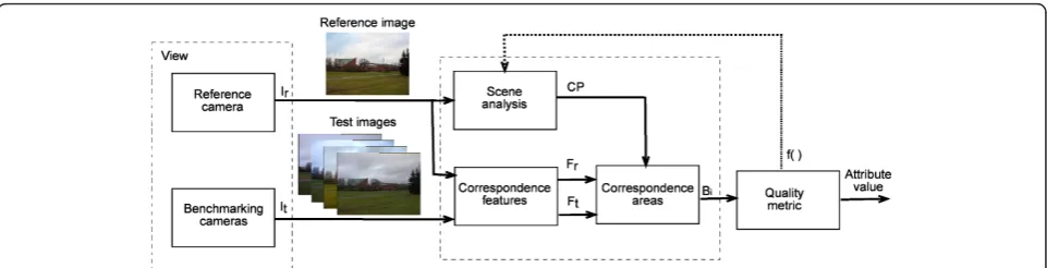
regions for the “Quality metric”component. This com-ponent includes the algorithm for computing the quality attribute in question. In this study, the quality attribute was sharpness. Section 3.5 describes the sharpness metric in detail. By changing the quality metric compo-nent algorithm, it is possible to use the reference-image framework for attributes other than sharpness.

The inputs to the framework are the reference imageIr

and the images captured with different cameras, called test imagesIt. Before the analysis, the reference and test

images are scaled to the same resolution. The“Scene analysis”component characterizes the scene using the reference image and selects candidate blocks for mea-surement. The output of the“Scene analysis”component is the vector of candidate points, CP, which includes the pixel coordinates of the so-called candidate blocks. The “Correspondence areas”component locates the blocks in the test images that correspond to the candidate blocks. This location is based on the correspondence featuresFr

andFtbetween the reference and test images. The

corre-spondence features are searched using the well-known SIFT algorithm (scale invariant feature transform). The SIFT algorithm is implemented in the“Correspondence features”component. The correspondence blocks (Bi,i=

1,2,...,m) are cropped from the test images and fed to the “Quality metric”component. Finally, the“Quality metric” component applies the attribute metric to the correspon-dence blocks.

The objective function,f(), is a feedback control of the “Quality metric” component. The objective function is used both for candidate block searching and the quality metric. In this study, the objective function was the stan-dard deviation of the wavelet coefficients. The dual task of the objective function is to locate the high-energy areas from the reference image and measure the corre-sponding areas’energy from the test images. The pro-posed reference-image framework is modular, and other quality attributes can be calculated by changing the objective function. The next subsections describe the components’functions in more detail.

3.2. Scene analysis

The“Scene analysis” component computes local values for the candidate blocks from the reference image using the function f(). It aims to find image areas with appro-priate structural energy for the quality attribute. The structural energy of the selected areas should change if a change in the quality attribute is perceivable. Smooth regions cannot be used for sharpness measurements because their energy levels can remain unaltered after some low-pass operations.

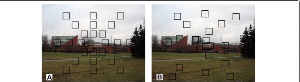
Figure 2a shows the initial points, IP, for finding local areas. The measurement blocks (M × M pixels) have been arranged in a predetermined symmetric order. The block-size parameter M is set to 100 pixels when the image size is 1600 × 1200 pixels. The initial symmetric order of the blocks in an image emphasizes the center area. The emphasis is based on the assumption that the important image objects and features often lie close to the center area. The framework samples the center area using more blocks than in the edge areas if the struc-tural energy of the center area is appropriate for the quality attribute in question. In Figure 2b, for example, the center area includes more candidate blocks than the edge area because of the high-energy trees in the center. The sharpness metric can use these high-energy trees.

A block becomes a candidate block if it maximizes the objective function in a limited neighborhood. The neigh-borhood size is determined by a tolerance value,T. Fig-ure 2b shows the candidate blocks whenT is 120 pixels and the image size is 1600 × 1200 pixels. Equation (3) shows the maximizing function used:

(CPy, CPx) = arg max CPy,CPx

⎛

⎝ 1

M2

j<CPy+M/2

CPy−M/2<j

k<CPx+M/2

CPx−M/2<k

x2_j_,_k

⎞ ⎠ (3)

CPyand CPxare the center coordinates of the block,

(5)

function d() computes a distance between the IP and CP. The IP are the center coordinates for the predeter-mined blocks. The CP are the center coordinates for the candidate blocks.

Figure 2b shows how the candidate block locations depend on the scene structure. Because Equation (3) maxi-mizes the first-scale wavelet energy, many candidate blocks include high-frequency structural objects, such as the trees in the image center. In this scene, the candidate blocks do not sample the strong edges between the roof and sky, as the higher-energy regions (trees) can be found in the neighborhood. The most important parameter of the method is the tolerance,T, which limits the size of the search window. Without tolerance, all measuring blocks would migrate to the highest-energy area of the scene. With tolerance, the sampling is more extensive, and the metric acquires more sampling points.

3.3. Correspondence features

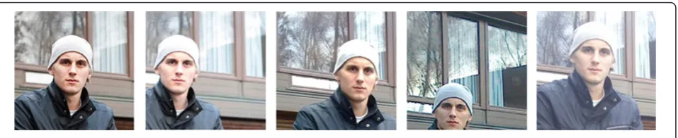
The output of the“Scene analysis”component contains candidate blocks. To measure the quality-attribute values for the test images, the blocks corresponding to the candi-date blocks in the reference images must be found in the test images. Locating the corresponding areas from the camera images is not a straightforward process, though the views of the reference and test images are the same. With the camera images, differences exist in features, including rotation, scaling, perspective, and brightness. Noise levels and types also differ. Figure 3 shows an exam-ple where images have been captured with different cam-eras so they are as similar as possible and the image regions have been cropped using the same pixel coordi-nates. It is obvious that correspondence block searching using only pixel-coordinate values does not work. A search using the block-correlation method also fails because of noise.

The proposed framework utilizes the SIFT method [42] for correspondence-block searching. The“Correspondence features”component computes feature vectors for the test

and reference images (Fr,Ft). The“Correspondence areas”

component locates correspondence blocks with the aid of the correspondence features. The SIFT algorithm was selected for the framework because SIFT-based methods are invariant to scaling, translation, and rotation, and they are partially invariant to brightness changes and perspec-tive [42]. In addition, the features are fairly robust to noise. The SIFT algorithm used [43] makes a scale-space transformation and calculates the difference of Gaussian (DoG) for the images at different scales. Local extremes are calculated by comparing the DoG sampling points to eight neighboring points in the same scale and nine neighboring points in higher and lower scales. The DoG point is a key point if its value is the highest or lowest in the neighborhood. Other points are excluded. Next, key points with low contrast or along an edge are excluded. Orientation histograms with 36 bins are calculated for the remaining key points. The orientation histogram is based on gradient orientations calculated from the sur-roundings of a key point after Gaussian filtering. The highest peak of the orientation histogram describes the key point orientation. If the histogram includes peaks with heights that are at least 80% of the highest peak, they are marked as the new key points for that direction. Finally, the point descriptors are defined. A key-point descriptor includes the orientation histograms from the neighborhood of the key point. In our imple-mentation, the descriptors have four orientation histo-grams with eight bins that describe the cell values for the feature vectors.

3.4. Correspondence areas

The SIFT algorithm was applied, and the 20 nearest cor-respondence features of the candidate block center in the reference image were used for the correspondence-block searching in the test images. The correspondence-block centers in the test images were located by calculating the angle and length of the vectors from the feature points to the candidate block centers in the reference image.

(6)

Figure 4 shows an example where eight correspon-dence features are used for the corresponcorrespon-dence-block searching in the test image. Figure 4a shows the candi-date block center and vectors from the correspondence features. Figure 4b shows the estimated block center for the test image. The estimate is based on the average of the vector end-points from the correspondence features.

3.5. Sharpness metric

The sharpness metric used in the reference-image fra-mework of this study is based on local energy. Local energy values are calculated as the standard deviation of the wavelet coefficients from the correspondence blocks located in the test image. The wavelet decomposition was performed using the MATLAB Wavelet toolbox. Based on pretest results, we elected to use only the first-scale diagonal coefficient values captured by the cameras selected for this study. We also elected to use Haar wavelets. In the pretest, vertical, horizontal, and diagonal sub-bands for the three scales were calculated. We tested single and different sub-band combinations using the same cameras and test images as in this study. The first-scale diagonal band proved to be the most robust. The objective sharpness metric for any correspondence blockBiwas computed from Equation (4):

Si=

1 (M−b)2

j<(M−b/2)

j>b/2

k<(M−b/2)

k>b/2

x2_j_,_k (4)

where the (j, k) are the pixel coordinates in a corre-spondence blockBi,M is the size of the correspondence

block Bi,b is a parameter for the reduced measurement

area, and xj, k is the diagonal wavelet coefficient. The

sharpness metric uses mcorrespondence blocks linked to the m highest-valued candidate blocks. The overall sharpness value is the average value of m correspon-dence blocks. In this study,mwas set between 1 and 24 when studying how the value ofmaffects performance.

The SIFT algorithm is robust and finds correspon-dence blocks well, but the corresponcorrespon-dence block edge areas can include structures from outside the original candidate-block area. The sharpness metric compensates for this inaccuracy with a reduced measurement area. If the candidate-block size used for block searching isM

pixels, the measurement area within the correspondence block in the distorted images is M - b pixels. In this study, the value of M was set to 50, 75, 100, and 125 pixels when studying how the value ofM affects perfor-mance. The value range of theMwas based on the pret-est. The parameter value ofb was set to 25 pixels.

4. Experimental settings for data collection

4.1. The image contents

The proposed method was validated using two datasets (Datasets I and II). Both datasets included five views (image contents). View contents were designed based on the photo space approach [44,45]. The photo space describes typical shooting distances and illuminance Figure 3Correspondence block searching using only the pixel-coordinate values is inaccurate.

(7)

levels for specific imaging-application areas. Our appli-cation was camera-phone benchmarking. By using two different datasets that were collected at different time periods, we were able to validate the robustness of the objective method.

The cameras for the tests were selected to cover a wide quality range: the selection consisted of low-, moderate-, and high-quality mobile phone cameras and moderate-quality compact cameras. The cameras’ pixel counts ranged from 3 to 12 Mpix. The views of Dataset I were captured by 13 cameras, and those of Dataset 14 cameras. In addition, all views were captured by a high-quality reference camera. The reference camera was a Canon EOS 5D with a Canon EF 24-80 mm lens. The performance (e.g., signal-to-noise ratio and detail reproduction) of the reference camera was considerably higher than that of the cameras to be tested, which was the only requirement.

Every view was captured several times by each camera. The cameras were set to their automatic mode, as the study benchmarked consumer products. The automatic mode is typically used by consumer photographers. Based on an expert evaluation, one image was selected to repre-sent each camera using the focus on the content target as the criterion. Images with a random white balance or exposure error were discarded.

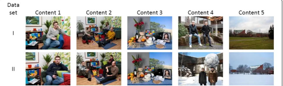
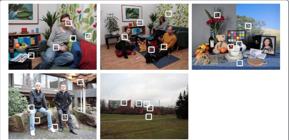
Figure 5 shows the image contents. The contents of Dataset I are shown on the upper row and those of Data-set II on the bottom row. Contents 1 and 2 simulate a living room environment. Content 4 simulates a tourist image, and Content 5 a landscape image. Contents 1, 2, 4, and 5 are views that mobile phone users can be expected to capture with their cameras. Content 3 is a studio image that device manufacturers use for signal-processing adjust-ments or other measureadjust-ments. The illuminances of Con-tents 1, 2, and 3 were 100, 10, and 1000 lux, respectively.

The most notable differences between Datasets I and II can be found in Contents 4 and 5. They were cap-tured outdoors in Finland, but in different seasons and

from different shooting positions. Dataset I was cap-tured in autumn and Dataset II in winter. The differ-ences in Contents 1 and 2 relate only to the people in the images and their clothes. Content 3 is identical for the two sets.

4.2. Subjective test settings

Because of the display size in the subjective tests, images were scaled to a size of 1600 × 1200 pixels. The interpo-lation method was bicubic. Black borders were also added around the images to match the image file and display resolutions (1920 × 1200). The test setup included two Eizo ColorEdge CG241W displays and a small display. The test images were shown on one dis-play one at a time, and the reference image (Dataset I) or several reference images (Dataset II) were shown on the other. The user interface included sliders for quality attributes and was mounted on the small display.

The observers first evaluated the overall quality value of a test image and selected the attribute values, one of which was sharpness. The other attributes were light-ness, saturation, and graininess. The continuous scale was from 0 to 100. All test images representing one content were shown sequentially. The order of the images and contents were randomized between the observers. Near visual acuity, near contrast vision (near F.A.C.T), and color vision were controlled before partici-pation. The viewing distance was approximately 80 cm, and the ambient illuminance was 20 lux. The displays were calibrated using the sRGB standard. We utilized the subjective sharpness data for this article. The follow-ing subsections describe the datasets’properties in more detail.

4.2.1. Dataset I

Dataset I included 65 test images (13 cameras × 5 con-tents). University students were used as observers (n= 25). They were all naïve with respect to image quality. Before the test, all test images and high- and low-quality

(8)

example images were shown to subjects at a rate of one second per picture. The reference image was shown on one display during the test, and the test images on the other display. The image-quality value of the reference image was set to 90 on a scale of 0-100. The reference image functioned as a high-quality anchor image. A quality value of 90 out of 100 left some latitude for the observers with high-quality test images. Reference images were tuned based on consumer preference expectations. Typical consumers prefer sharp, high con-trast, and colorful images.

4.2.2. Dataset II

Dataset II included 70 test images (14 cameras × 5 con-tents). University students were used as the observers (n

= 30). They were all naïve with respect to image quality. Before a single test image of a given content was shown, all test images of the content in question were shown to the observer as a slide show. This process was repeated before each test image was evaluated. We call this method a dynamic reference method. Before the test started, high- and low-quality example images were also shown to the observers. The main difference between Datasets I and II is that the observers saw all images of a given content before a single test image of Dataset II was assessed. Small differences between images were easier to find with this type of presentation. The differ-ences between the Datasets were motivated by the con-tinuous need to improve the procedures for subjective image quality testing.

4.3. Subjective sharpness data

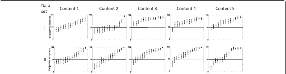
Figure 6 shows the content specific subjective sharpness values for Datasets I and II, sorted in ascending order. The 95% confidence intervals (vertical lines) and a sharpness value of 50 (horizontal lines) on a scale from 0 to 100 are added to the figures to aid comparisons. Based on Figure 6, there are clear differences in the scales of Datasets I and II. The scales of Dataset II are spread wider than those of Dataset I. This difference is

attributable to the data collection methods. Dataset II used the dynamic reference method. The observer saw all images representing one content before a single test image was evaluated. With Dataset II, the observer’s quality reference scale was thus based on the image set of the content under study. With Dataset I, the refer-ence was based more on the observer’s internal refer-ence because the referrefer-ence images were not shown during the test. An internal reference is known to be dependent on the observer’s individual experiences and memory.

Because the view and shooting environments were the same for both sets, Content 3 (the studio image) gives a good example of how the test method affected the data. The studio image is easy for cameras, as signal proces-sing in modern cameras can handle simple views. This consideration can be seen in the results achieved in Dataset I. The observers had difficulty seeing differences between the images. For Dataset II, the observers saw larger differences between the images. This distinction was due to the dynamic reference, which provided observers with a clear reference for the sharpness scale within the image set under consideration. Based on these results, the dynamic reference method functions well if differences are small but exist.

The problem with the dynamic reference method relates to content-specific normalization. Observers use content-specific anchors when quality values are given. The worst image from the content set functions as a low-quality anchor (quality value = 0), and the best image functions as a high-quality anchor (quality value = 100). We can expect that the same sharpness values for images of different contents would not be identical within Dataset II because some contents are more diffi-cult for cameras to detect than others. For example, the sharpness value of 50 for Content 3 is not the same as the sharpness value of 50 for the other contents. This effect should be considered when data are used for metric validation. Before Dataset II can be used, the

(9)

objective metric should be normalized in a content-spe-cific manner.

4.4. Reference images

We used two different reference image types: one for the subjective test (Dataset I) and one for the reference-image framework for the objective reference-image-quality metric. The difference between the reference image types arose from the image-processing aims. For the objective image-quality metric, image processing was minimized. Only the default algorithms of white balance, demosai-cing, and JPEG format compression were applied. The purpose was to characterize the views of Figure 5.

For the subjective test, the aim was to produce a pre-ferable image. In addition to the default algorithms, image sharpness, contrast, and colorfulness were adjusted according to known consumer preferences. These are assumed to favor sharp, high-contrast, and colorful images.

Figure 7 shows five candidate blocks for the reference images of Dataset I. The candidate blocks shown had the five highest sharpness values (m= 5), as calculated by Equation (3). The block size, M, is 100 pixels, and the image size is 1600 × 1200 pixels.

4.5. Other metrics

We compared the proposed method to the state-of-the-art NR, RR, and test-target metrics. Section 5.2 presents the results. The FR metrics were omitted from the per-formance analyses reported in Section 5.2; they would

not give meaningful results without additional pre-pro-cessing, as they require pixel-accurate alignment.

The NR sharpness metrics were from Marziliano et al. [29], Ferzli and Karam [30], and Narvekar and Karam [31], and the RR metric was from Wang and Simoncelli [18]. The NR metrics are local, and previous studies have reported their performance to be high [30,31]. The RR metric performance [18] was high in our pretest uti-lizing the test images captured by the different cameras in this study. We used the published code [46] for the Ferzli and Karam NR metric [30], the published code [47] for the Narveker and Karam NR metric [31], and the published code [48] for the Wang and Simoncelli RR metric [18]. We used Marziliano et al.’s [29] for the MATLAB implementation of their NR metric.

The RR metric [18] has been developed for overall image quality. The metric compares the wavelet coeffi-cient distributions between the reference and distorted images. Equation (2) calculates the overall image quality. Its high performance at predicting sharpness in our pretests relates to the correlation between image con-trast and wavelet coefficient energy. Image concon-trast relates to the perceived sharpness and detail reproduction.

In addition to the above algorithmic metrics, MTF50 values were calculated. The Mica test-target [49] images were captured under laboratory conditions. Low-illumi-nance lighting (100 lux) was used to simulate the condi-tions of Contents 1 and 2, and high-illuminance lighting (1000 lux) was used for the other contents. The Mica

(10)

target included low-contrast edges for the frequency-response calculations. A low contrast compensates for signal sharpening effects in cameras. The IE Analyzer v4.0.5 software was used for the calculations, and the reported values are for an average of ten test-target images.

5. Performance results

This section presents the performance of the proposed method. The proposed and other algorithmic methods were applied to the same interpolated image files used in the subjective tests. An interpolation algorithm can filter the images’structure and noise energy. Using the same interpolated image files for the objective metrics, we assessed the same images that the observers saw in the subjective study.

First, we analyzed the character of the proposed metric with different candidate-block sizes and different numbers of the correspondence blocks. Section 5.1 pre-sents these results. Based on these measurements, we selected the optimal settings for the performance com-parison between the proposed and the state-of-the-art metrics. Section 5.2 gives these results. Section 5.3 com-pares the performance of the proposed method for the Gaussian-blurred and JPEG2000-compressed images from the well-known LIVE database. The performance metrics were the Pearson linear correlation coefficient (LCC), Spearman rank-ordered correlation coefficient (ROCC), and root-mean square error (RMSE).

5.1. The influences of block size and number of blocks

The effects of the measurement-region size on the LCC values between the objective and subjective data were studied using measurement area sizes of 25, 50, 75, and 100 pixels. The candidate-block sizes were thus 50, 75, 100, and 125 pixels when located in the reference images. The reference camera’s candidate blocks were sorted in ascending order based on the objective func-tion value. Whenm= 1, the proposed sharpness metric used only the correspondence block of the candidate block with the highest sharpness (i = 1). When m= 2, the proposed sharpness metric used the correspondence blocks of the two highest-sharpness candidate blocks (i

= 1,2), and a similar pattern was used for other values ofm.

Figure 8a shows the average LCC plots of Datasets I and II as a function of the number of blocks for candi-date-block sizes of 50, 75, 100, and 125 pixels. The plots are the mean values over the contents before the non-linear fitting (Equation 5). Based on these results, block size has an effect on performance. The performance was highest when the candidate-block size was 100 pixels and the number of correspondence blocks was 5-8.

Figure 8b shows the LCC plots as a function of corre-spondence-block number, i. The proposed sharpness metric was calculated using a single correspondence block. The candidate-block size was 100 pixels. Based on Figure 8b, the selected correspondence block affects performance. The first clear decrease comes when i= 6. The second decrease comes when i = 21. The perfor-mance of five first blocks sorted by their Equation (4) values is thus high compared to the other blocks.

Based on these results, we concluded that the optimal candidate block size is 100 pixels and the optimal num-ber of blocks is 5. The candidate blocks were located using a block size of 100 pixels, and the measurement area inside the correspondence blocks was 75 pixels.

5.2. Comparison between the metrics

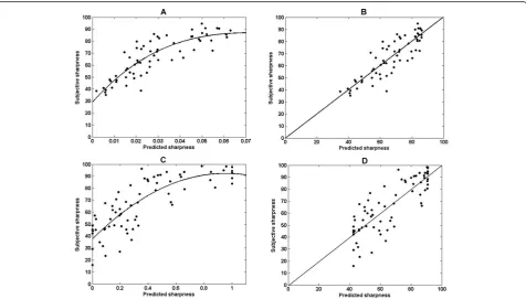
Figure 9a,c shows the subjective sharpness for Datasets I and II as a function of the proposed metric before the nonlinear fitting (Equation 5), and Figure 9b,d shows it afterwards. Figure 9a,c suggests that the relationship between the subjective and objective sharpness is non-linear. Because of the nonlinearity of subjective percep-tion, objective metric values should be fitted before drawing conclusions regarding performance. In this study, data from all metrics were fitted using the func-tion proposed by the VQEG report [50]:

Spred=

p1−p2

1 +e ⎛ ⎝vi−p3

p4 ⎞ ⎠

−p2

(5)

where p1,p2, p3 and p4 are fitting parameters of the

model, Spred is the predicted sharpness, and vi is the

metric value for imagei. The fitting parameters,pi, were

obtained by calculating the minimum least-squares, nonlinear regression using the fminsearch function in MATLAB.

(11)

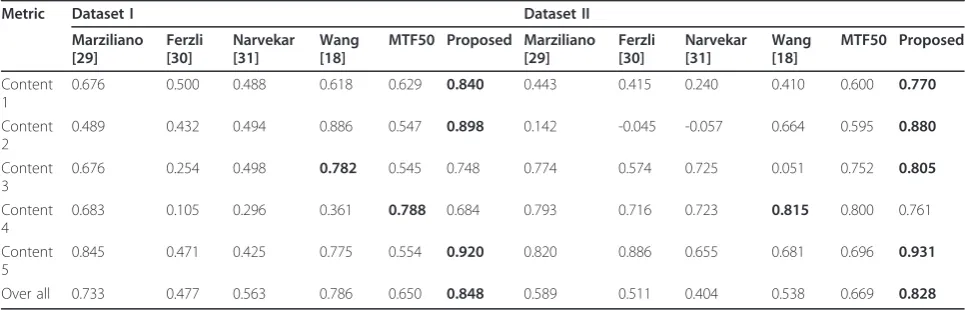
Based on Table 1 the performance of the proposed metric was higher than that of the previously published metrics. When the data were fitted over all contents, the LCC of the proposed metric was highest. The content-specific performance of the proposed metric was high-est, except for Contents 3 and 4 in Dataset I and Con-tent 4 in Dataset II. In these cases, the performance of the Wang and Simoncelli RR metric (Content 3 in Data-set I and Content 4 in DataData-set II) or the test-target MTF50 (Content 4 in Dataset I) was the highest.

Dataset II was more difficult for the proposed metric than Dataset I. Overall, the LCC for Dataset I was higher than for Dataset II; even the LCCs for Contents 3 and 4 in Dataset I were low compared to the other contents. Figure 9 shows the higher data dispersion of Dataset II compared to Dataset I.

Content independency was tested using the cross-vali-dation method. Datasets I and II were divided into five groups, each representing one content. The fitting para-meters of Equation (5) were estimated using data from Figure 8The average LCC of the proposed metric and the subjective sharpness.(a)LCC values for Datasets I and II as a function of the number of blocks,m, withM= 50, 75, 100, and 125.(b)The average LCC of the proposed metric as a function of the block number,i, whenM

= 100.

(12)

the four other groups. These four groups functioned as the training data. The fifth group was used as the valida-tion data. The validavalida-tion was performed five times. All groups (contents) functioned once as validation data. Table 2 shows the mean LCC, ROCC, and RMSE values of the proposed and Wang and Simoncelli RR metrics for the training and validation groups over all contents. In addition, the RMSE values are presented for the sub-jective data. The RMSE values for the subsub-jective data were calculated by comparing the single-observer values with the mean values for all observers of a content. Tables 3 and 4 show the content-specific LCC, ROCC, and RMSE values of the proposed and Wang and Simoncelli RR metric for the training and validation groups.

Tables 2, 3, and 4 show that the proposed metric per-formance was also high for the validation data. The mean performance was clearly higher than the Wang and Simoncelli RR metric performance. According to Tables 3 and 4, the content-specific LCC values for the proposed metric were higher than the LCC values of the Wang and Simoncelli metric, except for Content 3 in Datasets I and II.

The RMSE is the most interesting feature of the data. It indicates that the objective metrics outperform the subjective data metrics in predicting sharpness. This result mirrors nature and real problems relating to sub-jective data. In any case, it should be remembered that

goodness-of-fit type metrics, such as the RMSE, are fea-sible data-quality indicators only for objective data. The dispersion of subjective data may depend on the study material and instructions given. Subjective data should be handled as a probability distribution. It should be characterized and expressed using at least the mean and standard deviation.

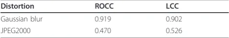
5.3. Performance using the LIVE image database

The LIVE database [51] contains 29 original images. The images are distorted using different distortion types and levels. The proposed metric was evaluated for the Gaussian-blurred and JPEG2000-compressed images. Table 5 shows the LCC and ROCC values for the pro-posed metric.

Based on the results, the performance for the Gaus-sian-blurred images is high and that for the JPEG2000-compressed images is lower. A reason for low perfor-mance of the JPEG2000 images can be the ringing dis-tortion because of heavy compression. The proposed method has not been developed for handling distortions of this type.

6. Conclusions

The analogy between the proposed and test-target meth-ods arises from using known image properties. Test-tar-get metrics determine the properties of test-tarTest-tar-get patches, and the proposed method can identify the Table 1 The LCC values of the benchmark metrics and the proposed metric with subjective sharpness.

Metric Dataset I Dataset II

Marziliano [29]

Ferzli [30]

Narvekar [31]

Wang [18]

MTF50 Proposed Marziliano [29]

Ferzli [30]

Narvekar [31]

Wang [18]

MTF50 Proposed

Content 1

0.676 0.500 0.488 0.618 0.629 0.840 0.443 0.415 0.240 0.410 0.600 0.770

Content 2

0.489 0.432 0.494 0.886 0.547 0.898 0.142 -0.045 -0.057 0.664 0.595 0.880

Content 3

0.676 0.254 0.498 0.782 0.545 0.748 0.774 0.574 0.725 0.051 0.752 0.805

Content 4

0.683 0.105 0.296 0.361 0.788 0.684 0.793 0.716 0.723 0.815 0.800 0.761

Content 5

0.845 0.471 0.425 0.775 0.554 0.920 0.820 0.886 0.655 0.681 0.696 0.931

Over all 0.733 0.477 0.563 0.786 0.650 0.848 0.589 0.511 0.404 0.538 0.669 0.828

Boldface indicates the best performer.

Table 2 The mean validation performance values for the metric [18] and the proposed metric.

Dataset Metric ROCC LCC RMSE RMSE (subjective)

Training Validation Training Validation Training Validation

I Proposed metric 0.838 0.781 0.843 0.811 8.812 10.241 20.737

Wang [18] 0.766 0.551 0.774 0.411 10.153 10.902

II Proposed metric 0.821 0.785 0.836 0.807 12.318 13.460 22.424

Wang [18] 0.577 0.635 0.630 0.576 16.407 19.195

(13)

properties of selected regions in natural images. The advantage of the test-target method is that the test images always contain areas with desired properties for the attribute of interest. The proposed method tries to find appropriate regions in the image. In some cases, performance can be lower if appropriate regions cannot be found in the image.

Based on the evaluation results, the proposed method is promising. The proposed method solves problems related to the NR, FR, and test-target methods. It con-siders image properties in a more advanced manner than the NR method. It can select the best areas of a scene based on quality attributes. For example, it does not try to interpret noise energy as image sharpness energy. Compared to FR methods, the proposed method does not require a pixel-wise reference image and is

thus applicable to performance studies of digital cam-eras, as in benchmarking camera phones. Compared to the test-target methods, the proposed method does not require the distinctly tedious process of preparing objec-tive test images. With the proposed method, the same natural images captured by cameras can be used for both subjective and objective measurements.

The proposed method predicts the perceived sharp-ness. The image-quality space of imaging devices is multi-dimensional. Sharpness is one low-level quality attribute. Other low-level attributes, including noise and color reproduction accuracy, are fairly simple to imple-ment in the proposed framework. Both can be measured using the same procedure, which locates the appropriate regions for measurement in the reference image using block data. Higher-level attributes, including naturalness and clarity, set higher requirements for the method. We can expect that new components need to be added in the framework. The higher-level attributes relate strongly to image content and semantics. The frame-work will require advanced computational methods for content understanding before higher-level attributes or overall image quality can be calculated.

Table 3 The content-specific validation performance values for Dataset I. Boldface indicates the best performer.

Content Metric ROCC LCC RMSE RMSE (subjective)

Content 1 Proposed metric 0.857 0.863 0.879 0.884 7.953 10.700 21.651

Wang [18] 0.783 0.692 0.814 0.625 9.711 12.818

Wang [18] 0.667 0.379 0.665 -0.484 10.677 8.907

Wang [18] 0.712 0.676 0.730 0.782 11.084 6.177

Wang [18] 0.835 0.209 0.829 0.362 9.746 12.450

Wang [18] 0.832 0.797 0.833 0.770 9.548 14.158

Table 4 The content-specific validation performance values for Dataset II.

Content Metric ROCC LCC RMSE RMSE (subjective)

Wang [18] 0.847 -0.275 0.838 -0.413 12.20 32.590

Wang [18] 0.499 0.829 0.591 0.761 16.79 18.620

Wang [18] 0.563 0.845 0.598 0.822 17.768 14.422

Wang [18] 0.527 0.877 0.587 0.829 17.78 14.699

Wang [18] 0.449 0.896 0.537 0.883 17.488 15.642

Boldface indicates the best performer.

Table 5 The evaluation of the proposed metric for images from the LIVE database

Distortion ROCC LCC

Gaussian blur 0.919 0.902

(14)

Acknowledgements

This study was partially supported by the Nokia Mobile Solutions/Symbian Smartphones. The authors thank Emeritus Professor Hannu Saarelma for reviewing the manuscript and Fredrik Hollsten and Jussi Tarvainen for the test images.

Author details 1

Department of Media Technology, Aalto University School of Science, P.O. Box 15500, FI00076 Aalto, Finland2_{Institute of Behavioural Science, University} of Helsinki, P.O. Box 9, FI00014 University of Helsinki, Finland

Competing interests

The authors declare that they have no competing interests.

Received: 26 October 2010 Accepted: 10 May 2012 Published: 10 May 2012

References

1. Sheikh HR, Sabir M, Bovik AC:A statistical evaluation of recent full reference image quality assessment algorithms.IEEE Trans Image Process

2006,15(11):3441-3452.

2. Lubin J:A human vision system model for objective picture quality measurements.Proceedings of International Broadcasting Conference

Amsterdam, Netherlands; 1997.

3. Wang Z, Bovik AC, Sheikh HR, Simoncelli EP:Image quality assessment: from error visibility to structural similarity.IEEE Trans Image Process2004, 13(4):600-612.

4. Sheikh HR, Bovik AC, Veciana G:An information fidelity criterion for image quality assessment using natural scene statistics.IEEE Trans Image Process

2005,14(12):2117-2128.

5. Yang C-L, Gao W-R, Po L-M:Discrete wavelet transform-based structural similarity for image quality assessment.Proceedings of IEEE International Conference on Image ProcessingSan Diego, CA, USA, 12-15 October 2008; 2008, 377-380.

6. Yang WY, Wu L, Fan Y, Wang Z:A method of image quality assessment based on region of interest.Proceedings of World Congress on Intelligent Control and AutomationChongqing, China, 25-27 June 2008; 2008, 6840-6843.

7. Geary B, Grecos C:Image quality assessment using a rotated gaussian discrimination function.Proceedings of Computer Vision and Pattern Recognition WorkshopSan Francisco, CA, USA, 13-18 June 2010; 2010, 47-52. 8. Li C, Bovik AC:Content-partitioned structural similarity index for image

quality assessment.Signal Process: Image Commun2010,25:517-526. 9. Tong Y, Konik H, Cheikh FA, Tremeau A:Full reference image quality

assessment based on saliency map analysis.J Imag Sci Technol2010, 54(3):030503.

10. Moorthy AK, Bovik AC:Visual importance pooling for image quality assessment.IEEE J Sel Topics Signal Process2009,3(2):193-201.

11. Engelke U, Zepernick H-J:Framework for optimal region of interest-based quality assessment in wireless imaging.J Electron Imag2010,

19(1):011005.

12. Meur OL, Ninassi A, Callet PL, Barba D:Over visual attention for free-viewing and quality assessment tasks. Impact of the regions of interest on a video quality metric.Signal Process: Image Commun2010,25:547-558. 13. Moorthy AK, Bovik AC:A two-step framework for constructing blind

image quality indices.IEEE Signal Process Lett2010,17(5):513-516. 14. Eerola T:Computational visual quality of digitally printed images.

Dissertation, Lappeenranta University of Technology; 2010.

15. Cui L, Allen AR:An image quality metric based on a colour appearance model.InAdvanced Concepts for Intelligent Vision Systems, ACIVS 2008. Volume 5259.Edited by: J Blanc-Talon, S Bourennane, W Philips, D Popescu, P Schenders. Springer, Heidelberg; 2008:696, France, 20-24 October 2008. Lecture Notes in Computer Science.

16. Radun J, Leisti T, Virtanen T, Häkkinen J, Vuori T, Nyman G:Evaluating the multivariate visual quality performance of image-processing components.ACM Trans Appl Percept2010,7(3):Article 16.

17. Leisti T, Radun J, Virtanen T, Halonen R, Nyman G:Subjective experience of image quality: attributes, definitions and decision making of subjective image quality.Proceedings of IS&T/SPIE International Symposium on Electronic Imaging 2009San Jose, CA, USA, 18-22 January 2009; 2009, 7242, 72420D.

18. Wang Z, Simoncelli EP:Reduced-reference image quality assessment using a wavelet-domain natural image statistic model.InProceedings of IS&T/SPIE International Symposium on Electronic Imaging 2005. Volume 5666.

San Jose, CA, USA, 17 January 2005; 2005:149-159.

19. Li Q, Wang Z:Reduced-reference image quality assessment using divisive normalization-based image representation.IEEE J Sel Topics Signal Process2009,3(2):202-211.

20. ISO 12233:2000(E). Photography_–Electronic still-picture cameras_– Resolution measurements. 2000, ISO.

21. ISO 15739:2003(E). Photography–Electronic still-picture cameras–Noise measurements. 2003, ISO.

22. ISO 17321-1:2006(E). Graphic technology and photography–Colour characterization of digital still cameras (DSCs)_–Part 1: Stimuli, metrology and test procedures. 2006, ISO.

23. ISO 14524:1999(E). Photography_–Electronic still-picture cameras_– Methods for measuring opto-electronic conversion functions (OECFs). 1999, ISO.

24. Koren N:The Imatest program: comparing cameras with different amount of sharpening.InProceedings of IS&T/SPIE International Symposium on Electronic Imaging 2006. Volume 6069.San Jose, CA, USA, 23 January 2006; 2006:195-203.

25. Okano Y:MTF Analysis and its measurements for digital still camera.In

Proceedings of IS&T 50th Annual Conference. Volume 50.Cambridge, MA, May 1997; 1997:383-387.

26. Loebich CM, Wueller D, Klingen B, Jaeger A:Digital camera resolution measurement using sinusoidal siemens stars.InProceedings of IS&T/SPIE International Symposium on Electronic Imaging 2007. Volume 6502.San Jose, CA, USA, 28 January 2007; 2007:65020N.

27. Artmann U, Wueller D:Interaction of image noise, spatial resolution, and low contrast fine detail preservation in digital image processing.In

Proceedings of IS&T/SPIE International Symposium on Electronic Imaging 2009. Volume 7250.San Jose, CA, USA, 18-22 January 2009; 2009:72500I. 28. Cao F, Guichard F, Hornung H:Measuring texture sharpness of a digital

camera.InProceedings of IS&T/SPIE International Symposium on Electronic Imaging 2009. Volume 7250.San Jose, CA, USA, 18-22 January 2009; 2009:27500H.

29. Marziliano P, Dufaux F, Winkler S, Ebrahimi T:Perceptual blur and ringing metrics: application to JPEG2000.Signal Process: Image Commun2004, 19(2):163-172.

30. Ferzli R, Karam LJ:A no-reference objective image sharpness metric based on the notion of just noticeable blur (JNB).IEEE Trans Image Process2009,18(4):717-728.

31. Narvekar ND, Karam LJ:A no-reference image blur metric based on the cumulative probability of blur detection (CPBD).IEEE Trans Image Process

2011,20(9):2678-2683.

32. Liang L, Chen J, Ma S, Zhao D, Gao W:A no-reference perceptual blur metric using histogram of gradient profile sharpness.Proceedings of IEEE International Conference on Image ProcessingCairo, Egypt, 7-10 November 2009; 2009, 4369-4372.

33. Caviedes J, Gurbuz S:No-reference sharpness metric based on local edge Kurtosis.Proceedings of IEEE International Conference on Image Processing

Rochester, New York, USA, 22-25 September 2002; 2002, 53-56.

34. Zhu X, Milanfar P:A no-reference sharpness metric sensitive to blur and noise.Proceedings of First International Workshop on Quality of Multimedia ExperienceSan Diego, CA, USA, 29-31 July 2009; 2009, 64-69.

35. Chen M-J, Bovik AC:No-reference image blur assessment using multiscale gradient.Proceedings of First International Workshop on Quality of Multimedia ExperienceSan Diego, CA, USA, 29-31 July 2009; 2009, 70-74. 36. Wee C-Y, Paramesram R:Image sharpness measure using eigenvalues.

Proceedings of Signal Processing, ICSP 2008Beijing, China, 26-29 October 2008; 2008, 840-843.

37. Sheikh HR, Bovik AC, Cormack L:No-reference quality assessment using natural scene statistics: JPEG2000.IEEE Trans Image Process2005, 14(11):1918-1927.

38. Zhang F-Y, Sun T, Tu YF, Qin Q-Q:Reduced reference image quality assessment based on wavelet domain singular value decomposition.In

Proceedings of IS&T/SPIE International Symposium on Electronic Imaging 2009. Volume 7498.San Jose, CA, USA, 18-22 January 2009; 2009:74984H. 39. Xue W, Mou X:Reduced reference image quality assessment based on

(15)

40. Cheng G, Cheng L:Reduced reference image quality assessment based on dual derivative priors.IEEE Electron Lett2009,45(18):937-939. 41. Nuutinen M, Orenius O, Säämänen T, Oittinen P:Reference image method

for measuring quality of photographs produced by digital cameras.In

Proceedings of IS&T/SPIE International Symposium on Electronic Imaging 2009. Volume 7867.San Jose, CA, USA, 17-21 January 2010; 2010:78670M. 42. Lowe DG:Distinctive image features from scale-invariant keypoints.Int J

Comput Vis2004,60(2):91-110.

43. Vedaldi A, Fulkerson B:VLFeat: an open and portable library of computer vision algorithms.[http://www.vlfeat.org], Accessed 15 Feb 2012. 44. CPIQ Phase 1 v.1.10. Camera Phone Image Quality–Phase 1–

Fundamentals and review of considered test methods. International Imaging Industry Association (I3A); 2007.

45. Segur RK:Using photographic space to improve the evaluation of consumer cameras.InProceedings of IS&T Image Processing, Image Quality, Image Capture, Systems Conference, PICS. Volume 3.Portland, USA, March 2000; 2000:221-224.

46. Ferzli R, Karam LJ:JNB Sharpness Metric Software.[http://ivulab.asu.edu/ Quality/JNBM], Accessed 15 Feb 2012.

47. Narvekar ND, Karam LJ:CPBD Sharpness Metric Software.[http://ivulab.asu. edu/Quality/CPBD], Accessed 15 Feb 2012.

48. Reduced-reference image quality assessment.[http://www.cns.nyu.edu/ ~zwang/files/research/rriqa/index.html].

49. Tervonen A, Nivala I, Ryytty P, Saari H, Ojanen H, Viinikanoja J:Integrated measurement system for miniature camera modules.InProceedings of IS&T/SPIE International Symposium on Electronic Imaging 2009. Volume 6196.

San Jose, CA, USA, 15-19 January 2006; 2006:61960L.

50. VQEG, Final Report from the Video Quality Expert Group on the Validation of Objective Models of Video Quality Assessment. 2000. 51. Sheikh HR, Wang Z, Cormack L, Bovik AC:LIVE image quality assessment

database release 2.[http://live.ece.utexas.edu/research/quality], Accessed 15 Feb 2012.

doi:10.1186/1687-5281-2012-8

Cite this article as:Nuutinenet al.:A framework for measuring sharpness in natural images captured by digital cameras based on reference image and local areas.EURASIP Journal on Image and Video Processing20122012:8.

Submit your manuscript to a

journal and benefi t from:

7Convenient online submission

7Rigorous peer review

7Immediate publication on acceptance

7Open access: articles freely available online

7High visibility within the fi eld

7Retaining the copyright to your article