http://www.sciencepublishinggroup.com/j/ajtas doi: 10.11648/j.ajtas.20190806.21
ISSN: 2326-8999 (Print); ISSN: 2326-9006 (Online)
Kriging and Simulation in Gaussian Random Fields Applied
to Soil Property Interpolation
Tofik Mussa Reshid
Department of Statistics, Werabe University, Werabe, Ethiopia
Email address:
To cite this article:
Tofik Mussa Reshid. Kriging and Simulation in Gaussian Random Fields Applied to Soil Property Interpolation. American Journal of Theoretical and Applied Statistics. Vol. 8, No. 6, 2019, pp. 296-305. doi: 10.11648/j.ajtas.20190806.21
Received: March 28, 2019; Accepted: October 24, 2019; Published: December 30, 2019
Abstract:
Spatial modeling is increasingly prominent in many fields of science as statisticians attempt to characterize variability of the processes that are spatially indexed. This paper shows that the Gaussian random field framework is useful for characterizing spatial statistics for soil properties. A sample of soil properties in 94 spatial locations are taken from a field (186.35m×211.44m) wide in northern Ethiopia, Karsa-Malima. We use observations of organic carbon (OC) from the site in our study. Box-Cox transformation is used because of OC follows non-Gaussian distributions. We develop ordinary kriging which is universal kriging with unknown trend models which enables us to predict any point within the field even outside the field up to the “Range” of the model. In this thesis work we predict 100×100 grids (10000 points) using kriging interpolation models. More over in each of these 10000 locations 1000 conditional simulations are made. Interestingly prediction using universal kriging and mean of conditional simulations agree in expectation and kriging variance. For covariance and/or variogram modeling and for parameter estimation we used least square principle and maximum likelihood estimation method. The classical geostatistical approach known as kriging is used as a spatial model for spatial prediction with associated spatial variances. Moreover, conditional simulation is performed. From ordinary kriging model results, predictions are accurate when predictions are close to observation locations. Prediction variance in the observed locations is close to the nugget effect.Keywords:
Gaussian Random Fields, Kriging, Interpolation, Variogram, Range1. Introduction
The concern of spatial variability in geostatistics is very important. Geostatisticians are mainly concerned with solving practical problems arise in the analysis of spatially correlated variables [1]. Observations indexed spatially have some pattern of correlation. Although not universally true objects in close proximity are more alike [2]. Knowledge of spatial variation of soil property is important in precision farming and environmental modeling [3].
The aim of this paper is to perform optimal prediction of soil property using kriging and Gaussian random field simulation. Soil property is the degree to which soil physical and/or chemical characteristics within a certain land use [4]. There is growing interest in modeling environmental effects of the agricultural sector [4]. Kriging and its derivatives constitute the most common class of spatial models used in diverse disciplines such as crop and soil science, geology, atmospheric science, and
more recently in ecology and the biological sciences [2]. Spatial variability is expressed by using variogram. Estimation of variogram parameters of soil properties using ordinary kriging is the general procedure to prepare soil maps [3].
The simulation employed in this paper is conditional simulation. The simulation is conditional on parameters of variogram and covariance models. An important part of spatial modeling is related to the speciation of the variogram/covariance structures; hence a discussion of this topic is included as well. Moreover, fitting variogram and/or covariance model of different families by comparing different methods is the other objective of this paper. This study focuses on modeling and predicting spatial soil properties using kriging based on Gaussian random field setup. The procedure for predicting the process is using interpolation of un-sampled locations.
with regression methods may improve prediction performance in comparison to regression or kriging done separately.
Modelling a process spatially indexed is useful for many purposes. One of the primary aim of spatial statistics is to infer spatially continuous surface over region of interest. This paper has provided a tool for how to analyze spatial process. It gives how to fit variogram model, how to perform kriging and simulation, how to predict spatially interpolated points in Gaussian random field. Since spatial statistics is relatively a new discipline this paper is a theoretical frame work and it gives how to model geostatistical process.
2. Methodology
We consider all observed values are outcomes of random variable observed at a given location. Let the random variable at a point in two-dimensional plane is
}
{
2( ) :
r s s∈ ⊆D R in our case D is two dimensional
( , )
D= x y . The process of interest ( )r si =ri is observed at n
locations s s1, 2,...sn
The aim is to predict the process r s( )0 =r0 in unobserved
locations0 =(x y0, 0). To predict the process in unobserved
locations we require covariance and variogram and certain assumptions related to the process
For two random variables ( )r s and ( ')r s the covariance function as defined in [5] is
( ( ), ( ')) [( ( ) ( ))( ( ') ( '))]
Cov r s r s =E r s −µ s r s −µ s (1)
The estimation of covariance function requires replication of observations. The standard method of obtaining replications is assumption of second order Stationarity (SOS). Observations cannot be made exactly at a point, but have to be average of volumes centered at each of these points [1]. Thus, we made SOS assumptions requiring three conditions [6].
i. E r s( ( ))=µ.
ii. Var r s( ( ))=σ2
iii. Cov r s r s( ( ), ( '))= Γ( )τ Where τ= −s s'
These conditions are constant mean and constant variance and the covariance between two variables is shift invariant and depends only on the spatial lag between them. τ= −s s'
The variogram function is defined as semi-variance.
( ( ) ( ')) 2 ( )
Var r s −r s = γ τ (2)
and ( )γ τ is called semi-variogram
For second order Stationarity γ τ( )= Γ(0)− Γ( )τ where (0)
Γ =covariance at zero spatial lag
If SOS is not hold we require another assumption. We need more general assumption requires to obtain replications. This assumption is called Intrinsic Stationarity (IS) [7]. This assumption requires two conditions:
i. E r s( ( )−r s( '))=0
ii. Var r s( ( )−r s( '))=2 ( )γ τ
That is the mean is constant and the variogram is depend only on
τ
and it is shift invariantThe advantages of IS over SOS are (1) to estimate variogram no estimation of µ is required (2) estimation of variogram is easier than covariance due to the sample estimator is unbiased (3) the variogram adapts more easily to more variability. (4) IS is more general assumption than SOS because, if SOS holds then IS also holds.
An assumption of constant mean may not achieve. Because sometimes variations occur in micro environments such as soil fertility and slope and etc. In this case the assumption of constant mean is naive because the neighboring observations tends to differ in property. In this case different trend of mean functions are taken
0 1 2
( )s x y
µ =β +β +β (3)
When the mean is linear on locations
2 2
0 1 2 3 4 5
( )s x y x y xy
µ =β +β +β +β +β +β (4)
When the mean is quadratic of locations
It is possible to denote in matrix form as
µ
=Sβ
. Where Sis a matrix of 1 in the first column and coordinate of locations or quadratic of coordinates in other column depending on the type of trend used and
β
is vector of regression parameters.Variogram and Covariance Models
By assuming IS or SOS to estimate these functions every pair of points separated by spatial lag
τ
gives an observed estimates (replications). The moment estimator of the samplevariogram γ τ( ) and sample covariance Γ( )τ , of
observations separated by lag
τ
are2
( , ')
1
ˆ( ) ( ( ) ( '))
2n s s N r s r s
τ τ
γ τ
∈
=
∑
− (5)and
( , ')
1
ˆ ( ) ([ ( ) )][ ( ') ])
s s N
r s r r s r
n τ τ
τ
∈
Γ =
∑
− − (6)Where
1
{( , ') : | ' | } and
n
i i
r
N s s s s r
n
τ = − =τ = =
∑
The moment estimator of the variogram is intuitive and unbiased. Still, there are two principal inadequacies of this estimator. The first stem is the variance must be positive. Consider any set of constants ai; i=1,...,n and spatial variable ( ); r si i=1,...,n it must hold that
1 1 1
( ) ( ), ( ) 0
n n n
i i i j i j
i i j
Var a r s a a Cov r s r s
= = =
= ≥
or analogously we require that
1 1
( ) 0
n n
i j i j
i j
a a
γ
s s= =
− ≤
∑∑
(8)The moment estimator does not satisfy the nonnegative definite property of the covariance function and the non positive definite property of the variogram function. The second reason, that the moment estimator inadequacy is that it gives estimates of correlation (covariance) only on observed spatial lags not for arbitrary lags. The common solutions to these difficulties are to fit valid parametric model.
Observations far away from each other do not have significant correlations. The correlation decays exponentially at the rate of decay parameter ϕ. i.e. the correlation vanishes
beyond lag distance R called range. For τ≥R ,
2
( ) (0)
γ τ = Γ =σ it is called sill. Then the correlation
parameters are the sill and decay parameter θ=(σ ϕ2, ) For SOS model if the covariance function is given then it is easy to express variogram function. This is not true for IS model, thus we need to express the variogram function. For now assuming isotropy i.e the correlation between observations at two locations depends only on the distance between them and not on the direction, or orientation, between them. And it must be positive definite.
( , ) [ ( ), ( ')]
(| |, )
anisotropic corr R s R s
isotropic
ρ τ θ ρ τ θ
=
(9)
The most common parametric families are Exponential model
2 || ||
( ; ) 1 exp τ
γ τ θ σ
ϕ
= − −
(10)
Gaussian model
2 2
( ; ) 1 exp τ
γ τ θ σ ϕ = − −
(11)
Spherical model
3 3 2
3 || || || ||
2 for || | |
2
( ; ) 2
else where τ τ σ τ ϕ ϕ γ τ θ ϕ σ − ≤ = (12)
For SOS model we consider 2
0 lim ( )
τ→ Γ
τ
=σ
[8] while0
lim ( ) 0
τ→ γ τ = . There are many cases these assumptions may not hold. Consider the following model
( ) ( ) ( ) ( )
R s =µ s +W s +ε s (13)
Where ( )µ s is the mean function, W s( ) is spatial random
perturbation and ( )ε s is noise term with Var( ( ))ε s =σn2
called nugget effect. Its alternative definition is
2 0
lim ( ) n
τ→
γ τ
=σ
and Cov( ( ), ( '))ε s ε s =0, for s≠s' then for this model the sill becomes2 2 2
r n
σ =σ +σ (14)
Where σ2 is called partial sill
Now the variogram (correlation) parameters are the partial sill the nugget effect and the decay parameter i.e
2 2
( , , n )
θ= σ ϕ σ Then the covariance function is
1 2
( , )τ θ ( , )τ θ ( , )τ θ
Γ = Γ + Γ (15)
Where
1( , )τ θ Cov W s W s( ( ), ( '))
Γ =
and
2( , )τ θ Cov( ( ), (ε s ε s τ))
Γ = +
Parameter estimation for variogram models
We must estimate appropriate model parameters for estimated variograms to find good kriging model. Let τ ={ ,... τ1 τm}
denote a set of m spatial lags where the variogram value were obtained and let γˆ={ ,... γˆ1 γˆm} denote obtained
non-parametric estimated variogram via moment, robust or kernel. Then we seek a parametric variogram function ( ; )γ τ θ which is closest to non-parametric estimate. The ordinary least square (OLS) estimate is choosing θ to minimize ( )Qθ equation 16
2 1 ˆ ( ) ( ( ; )) m i i
Qθ γ γ τ θ
=
=
∑
− (16)And the weighted least square (WLS) is to choosing θ to minimize Q( )θ in equation 17
2 2 1 ˆ ( ) ( ( ; )) m i i i
Qθ w γ γ τ θ
=
=
∑
− (17)Where wi2 is the diagonal elements of matrix W such that
1
ˆ
{ ( ( ; ))}
W = Var γ γ τ θ− − .
Gaussian Random field
For estimation of parameters and simulation of the process we
consider spatial Gaussian random field
{
R s s( ); ∈ ⊆D R2}
allfinite dimensional r=r s( )... (1 r sn) is multi-Gaussian
distributed with mean vectorµr, variance covariance matrix Σr
and isotropic correlation. Its density function is
(
)
1(
)
/ 2 1/ 2
1 1
( / , ) exp
2
(2 ) | |
r r n r r r
f r r r
r µ µ µ π − Σ = − − Σ −
Here µr =µ β( , )s is used for notation purpose is regression equation of the mean function as given in equation (3) or (4) and Σr is the variance- covariance matrix of the sill
has correlation parameters θ and Σr( )θ = Σ +σn2I where
Σmatrix of the partial sill and σn2is the nugget effect and I
is n dimensional identity matrix
Parameter estimation
The maximum likelihood of estimation method is
employed for this study. Given observations
1
( )... ( n)
r=r s r s the log likelihood is:
1
1 1
( ; , ) log(2 ) log | | ( ) ( )
2 2 2
T
r r r r
n
l r θ β = − π − Σ − r−µ Σ − r−µ (19)
Where µr the mean function as given in equation (3) or
(4). Then the maximum likelihood estimators are values that maximize the log likelihood function
( )
β θ,ˆ =arg maxβ θ, l r( ; , )β θ⌢
(20)
It is helpful to start by showing the optimization with respect to
β
treating θ as fixed. For fixed θ(
) (
1)
1 1
ˆ T T
r r
S S S r
β = Σ − − Σ − (21)
This estimator extends the OLS estimator to account the spatial correlation.
Similarly the numerical optimization of Newton Raphson iteration is used for θ by treating
β
as fixed1 2
1 1
2
( ) ( 1) j j
d d
j j l l
d d θ θ θ θ − − − = − −
(22)
Where θ θ= ( )j is the maximum likelihood estimator of θ for fixed
β
. The fisher scoring algorithm for optimum of log-likelihood with respect toβ
and θis(
( 1))
r θ j
Σ = Σ − , ˆ( )
(
T 1) (
1 T 1)
r r
j S S S r
β = Σ − − Σ −
and
1 2
2
( )j (j 1) E d l d l d d θ θ θ θ − = − −
Spatial prediction and simulation
The aim of this study is to perform spatial prediction using kriging and Gaussian simulation. Once the parameter of regression coefficients and correlation are estimated then to perform prediction is using covariance and semi-variogram models.
Let r is a vector of observed variables and we seek to
predict the process r0 at unobserved location s0. The joint
distribution is
0
0 02 0 0
~ 1 , r
r r Nn r r r µ σ µ Γ + Γ Σ
(23)
Sometimes the estimates are based on weights being associated to each observation. Consider a simple kriging model i.e the µ is known then the prediction at arbitrary location s0 =(x y0, 0)is
(
)
0 0 1 ˆ( ) n i i ir s µ α r µ
=
= +
∑
− (24)the prediction weights α =(α α1,... n) are determined by
minimizing kriging variance
{
0 0}
ˆ arg minα Var r(ˆ r )
α = − (25)
Hence
2 2 2
0
2 i i i j ij 0
i
d
dα σ α σ ρ α α σ ρ
− + =
∑
∑∑
(26)Solving for αˆ=(α1,...,αn)= Σ Γr−1 r0
Good estimation kriging weights using covariance function can be obtained when the trend parameters are known. If the trend parameters are unknown kriging weights in ordinary or universal kriging are obtained using variogram functions. Since knowledge of trend parameters is not required for variogram estimation. The aim is to minimize
2 0 1 n i i i
E αr r
=
−
∑
Subjected to1 1 n i i α = =
∑
By simplifying the term in the expectation and it is a function of
α
)
,...,
(
)
,
(
)
,
(
2
11 1 1
2
1
0 i j n
n i n i n j j i j i i n i i
i
r
r
s
s
s
s
F
E
α
=
α
γ
−
α
α
γ
=
α
α
Subjected to 1
1
( ,... ) 1 0
n
n i
i
Gα α α
=
=
∑
− =To solve this problem let m denote the Lagrange multiplier and set
( )
H α = −F mG
= 2 ( , ) − 2 ( , ) −
and
1
1
n
i i dH
dm =
∑
= α −Setting all n+1 derivative equal to 0 gives n+ 1 equation
with n+ 1 unknown. Soαi’s and m can be obtained by
solving the above equation. α = Γ−1γ where = ( , ) for all i and j and = ( , ) for all i
3. Result
The purpose of this study was to do spatial prediction by interpolation of unobserved locations using kriging and Gaussian simulation. Common type of spatial variogram models employed to estimate correlation parameters. We used the sample to predict the organic carbon (OC) content of a soil. The data was obtained at the office of National Soil Testing Center Addis Ababa, Ethiopia. The study area is located in northern Ethiopia, eastern Gojam. The area is 186.35m×211.44m. The data is a list of OC contents of soil in 94 locations of the field taken at depth 0-25 cm called top soil. Easting is referred to as “X-coordinate” and northing is “Y-coordinate”. “geoR” package in R-statistical software is employed for kriging, variogram fitting and spatial prediction [9, 14].
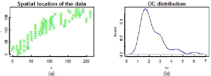
The spatial location and the density of OC is presented in Figure 1.
We start our data analysis by checking normality assumption. Figure 1 below describes the spatial location of the data and its distribution.
Figure 1. The sample data: (a) 94 spatial locations of the data, (b) The density of the OC.
The distribution in Figure 1 (b) shows the data is right skewed. Normality assumption was checked using Shapiro
Wilks test at 0.05 level of significance. The p-value of the test is very small, 8
2.58 10× − . Therefore, normality
assumption is failed and we need Box –Cox transformation to normality. Box cox transformed variable r' is
1
for 0
'
log for 0
r r
r λ
λ λ
λ
−
≠
=
=
We estimate Box-Cox transformation variable λ=0.65. Box-Cox transformed OC is plotted in Figure 2. Shapiro Wilks test is applied on transformed OC and the p-value is 0.35. Thus, we apply on transformed OC.
Figure 2 (a) shows the equality of the sample quantile and theoretical quantile and in (b) the transformed data is approximately normal. The p-value of the Shapiro Wilks test was 0.35.
Stationarity Diagnosis
The fundamental assumption in variogram estimation is intrinsic stationarity (IS) and second order stationarity (SOS). One of the assumptions of second order stationarity can be checked from the estimated residuals from the model that
best fits the trend function. The assumption of an SOS is appropriate when the trend function is smooth, since in kriging only relatively short spatial lags are used in prediction. Three models for the trend were evaluated; constant, linear and quadratic trends. The result of regression parameters along with model selection criteria was reported in Table 1. Estimation for coefficients of the trend with p-values, residual standard error (RSE), AIC and R2 are presented in the table.
Table 1. Parameter estimation for the trend in regression.
Trend Coefficients p-value RSE AIC R2
Cont. 0.55 2 10× −16 0.24 1.025 --
Lin. 0.76 1.83 10 1.5 10× -4 − × −3 7.25 10× −7 0.21 -19.4 22.9
Quad. 0.68 0.005 0.002 4 10− − × −5 6 10× −6 2 10× −5 1.3 10× −5 0.21 -19.4 24.39
In Table 1 the estimates of the coefficients in the linear and quadratic polynomial trends are very close to zero. The R2 is almost identical for all trend models. Moreover, the linear and quadratic trends add two and five additional parameters, but increases the log likelihood to only 10.21 and 12.21 respectively. This is not a significant improvement to the overall trend fit. Therefore, we conclude that the trend in the field considered was constant.
The second assumption of SOS can be checked from variogram. For second order stationary (SOS) field the semivariogram is bounded by the sill value as
τ
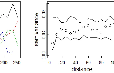
→ ∞(Bereke, 1999). In Table 1 we calculate RSE 0.24 and then the variance is 0.057, this is the sill. In Figure 3 (b) we computesemivariogram estimates with lag interval τ =4.7 m.
Variogram appears as bounded which shows they are SOS fields. In Figure 3 (b) the maximum variogram is 0.059 at maximum distance which is very close to the sill. This shows the second assumption for SOS is achieved.
For the data sets an assumption of weak Stationarity was achieved, next we need to asses isotropy and intrinsic stationarity (IS) of the data. Both of the assumptions can be assessed by graphical methods. Intrinsic isotropic stationarity will be checked using simulation of the data in a Gaussian random field. Variogram envelopes are computed assuming an intrinsic isotropic stationary Gaussian random field model. Simulated values were generated at the data locations, given
the model parameters. The empirical variogram was computed for each simulation using the same lags as for the original variogram of the data. The envelopes are computed by taking, at each lag, the maximum and minimum values of the variograms for the simulated data.
In our case, by taking 1000 stationary isotropic geo-data simulations, the envelop variogram was computed. Figure 3 (b) displays the semivariogram estimates in all bins are between the maximum and minimum semivariogram envelops. This shows the observed data were intrinsic stationary processes.
Kriging weights and variances are affected by anisotropy in the random field. Kriging weights become direction dependent as the degrees of anisotropy increase. Thus, we should evaluate whether the model satisfies the assumption of isotropy. The isotropic assumption of the spatial data can be checked by inspecting semivariogram function in different directions. In our
case we select four directions (0, , , 3
4 2 4
π π π
) to fit the
semivariogram. Figure 3 (a) displays the moment method estimated variogram of the transformed data. Variogram values were computed in four direction for lag parameter τ=4.7m. The maximum distance taken was 100m to estimate the
Figure 3. Variogram for the data: (a) directional variogram (b) variogram envelope.
Estimation and fitting Variogram function
The variogram function is the main tool in the analysis of spatial data. The variogram function of the residuals deviated from one observation to the other was estimated. Two ways of estimating the variogram function was used in this study: the moment method with least square fit and the maximum likelihood estimation. To estimate the variogram we first divide the data into different lag bins based on their location. The computation of the empirical variograms were under the assumption of second order stationarity (SOS). The
parameters of the variogram models are estimated by both ordinary least square (OLS) and weighted least square (WLS).
The trend was assumed to be constant, hence unbiased estimates of variogram estimates were obtained. Table 2 shows parameter estimates of three variogram models estimated from residuals of the trend. The estimates were based on minimizing sum of squares errors (MSS) for OLS and minimizing weighted sum of squared error (WSS) for WLS.
Table 2. OLS estimates of variogram parameters.
Cov. model OLS WLS
φ R MSS φ R WSS
exponential 0.0508 7.7 0 23.27 7.3×10⁻⁴
0.041 6 0.009 14.3 42.6
Gaussian 0.05 8.18 0.002 14.16 7.3×10⁻⁴
0.041 8.29 0.01 14.34 43.59
spherical 0.0455 21 0.0019 21 6.5×10⁻⁴ 0.046 21 0.009 21.42 46.94
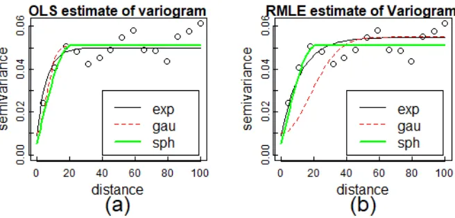
From Table 2 and Figure 4 (a) we observe that in all empirical variogram models the OLS and WLS estimates have good agreement in terms of the sill value (i.e σ2+σn2). We observe
that the nugget effect is equal to zero for the OLS estimate. For the WLS estimate it seems appropriate to allow a small nugget effect for transformed OC. Since the number of observations vary from lag to lag, we trust the WLS estimates more than the OLS estimates. The exponential model has small rate of decay (ϕ ) and hence it has large range (R) which enables us to perform Krigink more distance away from the observed
locations than other models. The exponential variogram was preferable because of that it has the least weighted sum of residual squares (WSS) for transformed OC hence it is used in the rest of the study.
Using variogram parameter estimates in least square principle we fitted the variogram functions. In Figure 4 (a) the moment method variogram estimates of the data with OLS and WLS fitted variogram functions are displayed and Figure 4 (b) shows restricted maximum likelihood fit for moment estimate of variogram.
Figure 4. Estimated variogram and fitted model: (a) OLS estimate, (b) RMLE estimate.
The variogram function is also estimated using maximum likelihood. The Transformed OC observations are found to be compatible with normality. Thus, it is reasonable to assume that the data come from jointly normal distributions. By using maximum likelihood estimation the trend and three types of variogram model parameters are estimated. We are actually using restricted maximum likelihood estimation
(REML) to estimate the parameters (in Table 3) and the fitted model were shown in the above Figure 4 (b).
In Table 3 the parameter estimates of the constant trend, the exponential, Gaussian and spherical variogram models are presented with model selection criteria AIC and BIC. Also the efficient range (R) of the variogram function is given.
Table 3. REML estimates of trend and variogram parameters.
Cov. model β φ R AIC BIC
Exponential 0.535 0.0458 11.37 0.013 34.05 -9.98 0.2
Spherical 0.5435 0.045 24.7 0.012 24.7 -8.05 1.54
In REML fits, unlike OLS and WLS fits, the nugget effect is appeared for all variogram models.
The moment estimates in Table 2 and the REML estimates in Table 3 are in a little beat agreed. It seems appropriate to allow a small nugget effect. Due to the increase in the nugget values the range of the correlation function obtained in REML are increase compared to the ranges computed in OLS and WLS fits. Exponential model is found to be smaller in AIC and BIC values, therefore, we used exponential model for kriging.
Kriging and Simulation
By using the assumption of spatial isotropic stationary random field and using the estimated variogram models we can predict the transformed OC surfaces and compute the associated variance of predictions. Ordinary kriging, which corresponds to universal kriging with an unknown constant trend, was used to predict and to compute kriging variance. In Figure 5 ordinary kriging predictions on a regular 100×100 grid over [0, 200]×[0, 200] covering the area conditional on the 94 sample data for transform OC are displayed.
Figure 5. Kriging interpolation: (a) predicted transformed OC (b) kriging variance.
Predictions near to the observed location are very similar to the observed values. And There is a correlation between predicted values near each other. As the distance far away, the correlation vanishes exponentially.
In figure 5 (b) the kriging variance shows the kriging variance is zero for predictions in observed locations. And the variance increases as predictions for distance far from observed locations. The kriging variance is small in the range (R) and grows to the sill (nugget plus partial sill) beyond R.
Simulation provides realizations of the Gaussian random
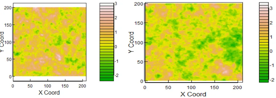
field conditioned on the 94 sample data. Based on the observed data estimated model parameters we take 1000 simulations of for each of ten thousand locations the surface for OCb. Figure 6 display two conditional simulations. Note that the observations are reproduced to the observed precession and that the variability is according to the estimated variogram models in Gaussian random field. Hence the conditional simulations in Figure 6 are more variable than the kriging predictions in Figure 5.
Figure 6. Two simulations 100X100 grid over prediction is done.
Figure 7 displays the average of 1000 conditional simulations and the variance of 1000 conditional simulations
observations, and is similar to the trend values far away from the observation locations. In Figure 6 (right) it reproduces the kriging variance in Figure 5. Note that the variance in the
observation locations is close to zero, while it is close to the sill value far from observation locations.
Figure 7. Average of 1000 simulations (left), Empirical variance of 1000 simulations (right).
Crossvalidation
The kriging predictor is an exact interpolator in the sense that the observed values are reproduced if no observation errors are present. Crossvalidation is done by leaving one observation out and predict the value in the associated
location using the remaining observations. The
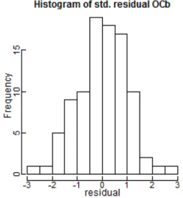
crossvalidation error is the observation minus the prediction. In Figure 8 the cross validation errors are displayed.
The crossvalidation error is approximately normally distributed with mean zero. The observed vs the predicted values lie approximately in the straight line that they show correlation 0.58. Using Pukelsheim theorem all predicted values are approximately within 96.66% confidence interval i.e. the p-values of the model is 0.034.
Figure 8. Histogram of cross validation errors in 94 observations.
4. Discussion
The main aim of geo statistics is to model a continuous
spatial variation [13]. Recently there has been an increasing interest in modelling spatial data [18, 20]. In this paper modelling includes making prediction and finding unbiased estimate of regionalized variable. The regionalized variable regarded as the most widely used realization Gaussian random field [10-12]. In this paper we predict unsampled location by interpolation [22, 23]. The prediction requires assumption of isotropic stationary Gaussian process, that is achieved after transformation. One way of finding optimal prediction of regionalized variable at unsampled location is through kriging [13, 15-17, 19]. Kriging is a technique of making optimal, unbiased estimate of regionalized variable at unsampled location using theoretical semivariogram [13, 24]. Variogram that gives minimum squared error is chosen for prediction and kriging variance. The main idea of kriging is that near sample points should get more weight in prediction. Kriging variance are close to the nugget effect near to observed data location and it grow to the sill as prediction location far apart from observed data location [21]. The kriging variance of the prediction is smaller than the observed sample variance. This is due to prediction is done in Gaussian random field.
5. Conclusions
simulation. As expected, kriging predictors are more accurate when the predictions are close to the observation locations. The variance of the predictors increases with increasing distance from observation locations. Moreover, conditional simulations using the Gaussian random field model is made. There is a relationship between kriging and conditional simulations since the average of the conditional simulations corresponds to the kriging surface while the variance of simulations corresponds to kriging variance. The effect is demonstrated in the study. Kriging predictors are accurate while the cross-validation errors should be normally distributed with mean zero and this is demonstrated.
References
[1] Omre H.; 1984: Introduction to Geostatistical Theory and Examples of Practical Application; Note, pp. 1-20.
[2] Wikle C. K, and Royle J. A; 2010: Spatial Statistical Modeling in Biology, Encyclopedia of Life Support System (EOLSS), Eolss Publisher, [http://www.eolss.net] (accessed on 11, 2011), pp. 1-27.
[3] Santra P, Chopra U. K and Chakraborty D; 2008: Spatial variability of soil properties and its application in predicting surface map of hydraulic parameters in an agricultural farm, Current science, Vol. 95, No. 7, pp. 1-9.
[4] Kempen M, Heckelei T, Britz W, Leip A, Koeble R, Marchi G; 2005: Computation of a European Spatial Land Use Map the Underlying Statistical Procedures; Agricultural and Resource Economics, Discussion Paper, pp. 1-16.
[5] Bohling G; 2005: Kriging, C and PE 940, Note, [http://people.ku.edu/∼gbohling/cpe940] (accessed on 3, 2012); pp. 1-20.
[6] Alan E. G, Peter J. D, Montserrat F. and Petter G.; 2010: Hand Book of Spatial statistics; Modern Statistical Method; Chapman and Hall.
[7] Chiles; J-P. and Delfiner P; 2012: Geostatistics: Modeling Spatial Uncertainity; 2.
[8] Matheron G.; 1965: Les Variables Regionalisees of lear Estimation. Une Application de la Theorie des Functiones Alatoires aux science de la Natwe; Masson, Paris.
[9] Paulo J. Ribeiro and Peter J. Diggle; may 2, 2016: analysis of geostatistical data; version1.7-5.2.
[10] Kevin P Murphy; 2007: Conjugate Bayesian Analysis of the Gaussian Distribution; Note; pp. 1-29.
[11] Simpson D, Lindgren F and Rue H; 2011: Markovian Gaussian Model in Spatial Statistics; Statistics, No. 9, pp. 1-17.
[12] Rue H and Martino S; 2006: Approximate Bayesian Inference for Hierarchical Gaussian Markov Random Field Models, Statistical Planning and Inference, Vol. 137, pp. 1-8.
[13] Vijay Kumar and Remadevi; 2006: Kriging of Ground Water Levels-A Case Study; Journal of Spatial Hydrology Vol. 6 No. 1.
[14] Paulo J. Ribeiro and Peter J. Diggle; 2001: geoR: A Package for Geostatistical analysis, Vol.1/2.
[15] Firas Ajil Jassim, Fawzi Hasan Altaany; 2013: Image Interpolation Using Kriging Technique for Spatial Data; Canadian Journal on Image Processing and Computer Vision Vol. 4 No. 2.
[16] Andreas Lichtenstern; 2013: Kriging Method in Spatial Statistics; Bachelor’s Thesis.
[17] Rue H and Follestad T; 2003: Gaussian Markov Random Field Models with Applications; Spatial Statistics; pp. 1-20. [18] Gao Gu M and Zhu H; 2000: Maximum Likelihood
Estimation for Spatial Models by Markov Chain Monte Carlo Approximation; J. R statist.soc.; Vol. 63, part 2, pp. 339-355. [19] Ethan B and Michael L; 2008: Estimating Deformations of
Isotropic Gaussian Random Fields on the Plane; The Anals of Statistics; Vol. 36, No. 2,; pp. 1-24.
[20] Jo Eidsvik; 2011: Spatial statistics, Parameter Estimation and Kriging for Gaussian Random Fields; Note, pp 1-12.
[21] Michael Sherman.; 2011: Spatial Statistics and Spatio-Temporal Data, Covariance Function and Directional Properties; Jhon Wiley and sons Ltd publication
[22] Derya Ozturk and Fatmagul Kilic; 2016: Geostatistical Approach for Spatial Interpolation of Meteorological data; Anal of the Brazilian Academy of science.