M E T H O D O L O G Y
Open Access
A new multivariate two-sample test using regular
minimum-weight spanning subgraphs
David M Ruth
Correspondence:[email protected] Department of Mathematics, United States Naval Academy, 572-C Holloway Rd, Annapolis, MD 21402, USA
Abstract
A new nonparametric test is proposed for the multivariate two-sample problem. Similar to Rosenbaum’s cross-match test, each observation is considered to be a vertex of a complete undirected weighted graph; interpoint distances are edge weights. A minimum-weight, r-regular subgraph is constructed, and the mean cross-count test statistic is equal to the number of edges in the subgraph containing one observation from the first group and one from the second, divided byr. Unequal distributions will tend to result in fewer edges that connect vertices between different groups. The mean cross-count test is sensitive to a wide range of distribution differences and has impressive power characteristics. We derive the first and second moments of the mean cross-count test, and note that simulation studies suggest this test statistic is asymptotically normal regardless of underlying data distributions. A small simulation study compares the power of the mean cross-count test to Hotelling’sT2test and to the cross-match test. This new test is a more powerful generalization of Rosenbaum’s test (the cross-match test is the caser= 1) and constitutes a noteworthy addition to the class of multivariate, nonparametric two-sample tests.
Keywords:Distribution-free test; Graph-theoretic procedure; Change point
1 Background
1.1 Objective
Consider N=m+nindependent multivariate observationsY1, …,Ymand Ym+ 1, …,YN,
where eachYiis drawn from distributionFfor 1≤i≤mand from distributionGform+
1≤i≤N. The dimension of the observations does not depend onN.The covariates may be quantitative or categorical; there need only exist some function,d, that measures dis-tance between observations. The null hypothesis is that F=G. The objective is a two-sample test that has little or no dependence on the underlying distribution of the data. Furthermore, this test should have sufficient power to be useful for applications.
1.2 Motivation
We follow in the vein of graph-theoretic tests for homogeneity: Consider each observation to be a vertex of a complete, undirected, weighted graph,G, and assign interpoint distances as edge weights. The distribution of these distances is sensitive to departures from homo-geneity; Maa et al. (1996) prove that two distributions are identical if and only if the distri-butions of inter-point distances within and between observations sampled from the two populations are the same. Friedman and Rafsky (1979, 1981) fit a minimum spanning tree
toGand count the number of edges in the tree that connect vertices from different groups to test whether the sampling distributions are the same. Schilling (1986), Henze (1988), and Hall and Tajvidi (2002) examine properties of nearest-neighbor subgraphs of G to test for homogeneity.
Rosenbaum (2005) provides a novel approach to this problem: Suppose N is even. Find a minimum-weight non-bipartite matching onG, which is the lowest-weight span-ning subgraph for which the degree of each vertex with respect to the subgraph is one and which consists of N/2 non-adjacent edges. Rosenbaum’s cross-match statistic, A1, counts the number of edges in the matching that include one vertex from each of the two groups. Under the null hypothesis of no group difference each vertex is equally likely to be paired with any other vertex. Rosenbaum (2005) shows that the exact null distribution ofA1is found by combinatorial argument to be
P Að 1¼a1Þ ¼
2a1ðN=2Þ! N
m m−a1
2
!a1!
n−a1
2
!
ð1Þ
for a1∈{0, 2,…, min(m,n)} andm andneven, ora1∈{1, 3,…, min(m,n)} andm andn odd; P(A1=a1) = 0 otherwise. In the denominator of (1), 12ðm−a1Þ is the number of edges in the matching where both vertices are in the group of size mand 1
2ðn−a1Þ is the number of edges in the matching where both vertices are in the group of sizen.
When the two groups are drawn from different distributions the number of within-group pairs tends to be higher than for the null case, so the null hypothesis of homo-geneity is rejected if A1is sufficiently small. For oddN, this procedure may be simply modified by introducing a pseudo-observation, Y0such thatd(Y0,Yi) = 0 for all i∈{1,
…,N}, and randomly assigning it to one of the two groups. Then find a minimum-weight non-bipartite matching on this resulting graph with N+ 1 vertices and compute A1with respect to observationsY0,…,YN.
That the exact null distribution of A1is known, regardless of the underlying data dis-tribution, is a particularly attractive property for a multivariate two-sample test. Fur-thermore, the asymptotic normality of A1facilitates testing for large-sample problems. However, the cross-match test has relatively low power. Since only a single non-bipartite matching is considered in this test, information contained in the proximity of many pairs of points is ignored. Friedman and Rafsky (1979, 1981) observe that the power of their single-tree test is enhanced by evaluating successive disjoint low-weight spanning trees. Similarly, Ruth and Koyak (2011) show that ensembles of disjoint low-weight non-bipartite matchings carry significant information regarding whether a distri-butional change occurs over a sequence of independent observations. A drawback asso-ciated with examining collections of such subgraphs is that null distributions are extremely difficult to determine. Mindful of this caveat, we offer an extension of the cross-match test which exploits the information contained in the distances between many pairs of points.
2 Methods
2.1 Illustrating example
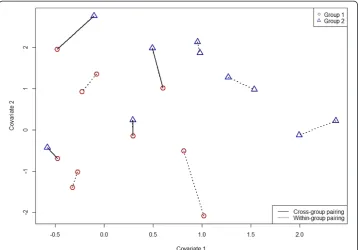
within groups are identically distributed. For the purposes of this example, these data were simulated from distributions whose locations differ by one unit in each dimension. Figure 1 also shows the minimum-weight non-bipartite matching associated with this sample with respect to Euclidean distance. The present goal is to identify the distribution difference be-tween these groups, making no assumptions about the underlying distributions.
The cross-match test is applicable here; for this example the value of the cross-match statistic is A1= 4 with a corresponding p‐value = 0.433. So, the cross-match test is in-sufficiently powerful to identify a distribution difference in this case. In the next sec-tion, we introduce an extension of the cross-match test that enhances test power significantly.
2.2 The mean cross-count (MCC) test
As before, we assume an even numberNof observations forming a complete, undirected, weighted graph,G. Rather than find a minimum-weight non-bipartite matching, we find a minimum-weight r-regular spanning subgraph of G, where 1≤r≤N−2, denotedGr. That is,Gr is a subgraph ofGwith the following properties:
a) Every vertex inGis also inGr. b) Every vertex inGr has degreer.
c) The total weight of all edges inGr is the lowest among all subgraphs ofGwhich satisfy properties (a) and (b).
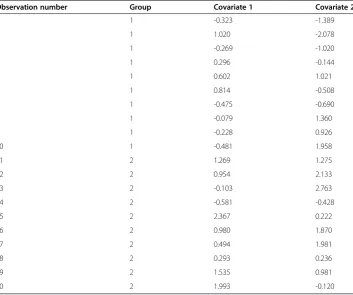
Table 1 Bivariate data for illustrating example
Observation number Group Covariate 1 Covariate 2
1 1 -0.323 -1.389
2 1 1.020 -2.078
3 1 -0.269 -1.020
4 1 0.296 -0.144
5 1 0.602 1.021
6 1 0.814 -0.508
7 1 -0.475 -0.690
8 1 -0.079 1.360
9 1 -0.228 0.926
10 1 -0.481 1.958
11 2 1.269 1.275
12 2 0.954 2.133
13 2 -0.103 2.763
14 2 -0.581 -0.428
15 2 2.367 0.222
16 2 0.980 1.870
17 2 0.494 1.981
18 2 0.293 0.236
19 2 1.535 0.981
In graph theory, an r-regular spanning subgraph of Gis sometimes called anr-factor ofG. Note thatG1is the special case of a minimum-weight non-bipartite matching used by Rosenbaum (2005), and GN−1 is identical toG. In practice, we are mainly interested in 2≤r≤N/2, although the theoretical details are not so constrained. Minimum-weight r-factors may be computed as follows: For any subgraph of G, let xij be an indicator
variable equal to 1 if the edge connecting vertices i andjis included in the subgraph and letdijbe the distance between vertexiand vertexj. Then the edges ofGr solve
fol-lowing the combinatorial optimization problem:
minx XN
j¼2
Xj−1
i¼1 dijxij
subject toX k−1
i¼1
xikþ X N
j¼kþ1
xkj¼r ∀k∈f1;…;Ng
xij∈f0;1g∀j∈fiþ1;…;Ng; ∀i∈f1;…;N−1g:
ð2Þ
Anderson (1972) assures the existence of a solution forr≤N/2. Solutions forr>N/2 are guaranteed by the fact that the complement of an r-regular subgraph of G is an (N−1−r) -regular graph. For this paper, solutions are found in R using the package “lpSolve” for N≤400. For N> 400, solutions are found in R using the package “gurobi” due to the computational complexity of larger problems.
Similar to the cross-match test, we count the number of edgesArinGr that include a
vertex from each group. We call Tr =Ar/rthe mean cross-count (MCC)statistic. The
idea here is that the number of within-group edges in Gr will be higher for cases of a distribution difference than for the null case. So, small values ofTrare evidence against
the null hypothesis. Note that T1=A1is the cross-match statistic as before. One could use the total cross-count, Ar, as an equivalent test-statistic; however, we choose to scale
this value to give some notion of “average cross-count per vertex degree” (hence the name“mean cross-count”). For oddN, randomly introduce a pseudo-observation in the same manner as ther= 1 case discussed in Section 1.2.
2.3 Illustrating example, continued
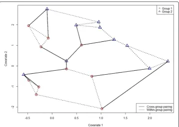
Figure 2 shows a minimum-weight 3-factor, G3, for the data in Table 1 with respect to Euclidean distance. Cross-group edges are shown with solid lines. For this case, A3= 12⇒T3= 4, so the test statistic value here is the same as Rosenbaum’s cross-match test statistic. A discussion of the distribution ofTris in Section 3.1; for this example, we
es-timate the p-value for Tr by permutation test on the observation vertex labels. Using
10,000 permutations yields an estimated p‐value = 0.146. While not enough evidence to conclude a group difference, this reduction in p-value relative to the r= 1 case (p-value = 0.433) suggests that considering minimum-weight r-factors for r> 1 may improve test power. In Section 3.2 we demonstrate significant power advantages that are realized for the MCC statistic.
3 Results and discussion
3.1 MCC moments and normal approximation
For the following discussion we assume Nis even, adopting the convention that if the number of observations is odd then we will consider Nto be the number of observa-tions including a pseudo-observation as previously discussed. To find the mean and variance of Trunder the null hypothesis, we proceed as follows: Let Gbe the complete
undirected graph (ℤN,EN) where the vertex setℤNconsists of the indices 1, 2,…,Nand
the edge set consists of all N(N - 1)/2 pairs of vertices; by convention, write the pairs with smaller vertex first, soEN= {(i,j) : 1≤i<j≤N}. Partition ℤNinto two setsS andT,
with |S| =mand |T| =n, so m+n=N. Denote EðNS;TÞ as the set of all edges with one vertex in S and the other in T. Let Xij be the random variable that indicates whether
edge (i,j) is included in a minimum-weight r-regular subgraph, Gr, with 1≤r≤N−2.
By ther-regularity ofGr, for eachi∈ℤNwe haver¼
Xi−1
j¼1
Xjiþ XN
j¼iþ1
Xij;and so
r¼E r½ ¼ E X i−1
j¼1 Xjiþ
XN
j¼iþ1 Xij
" #
¼Xi−1 j¼1
E Xji þ XN
j¼iþ1 E Xij
¼Xi−1 j¼1
P Xji ¼1þ X N
j¼iþ1
P Xij ¼1:
ð3Þ
But under the null hypothesis, each edge is equally likely to be included inGr, so r= (N−1)P(X12= 1). Therefore, for all (i,j)∈EN
E Xij ¼ P Xij ¼1¼ r
N−1 ð4Þ
and
Var Xij ¼P Xij¼1
P Xij ¼0¼r Nð −1−rÞ N−1
ð Þ2 : ð5Þ
The total cross-count,Ar, may be written
Ar¼ X
i;j ð Þ∈EðNS;TÞ
Xij ð6Þ
resulting in
E T½ ¼r 1 rE A½ ¼r
1 rE
X
i;j ð Þ∈EðNS;TÞ
Xij 2 6 4 3 7 5¼mn
r E Xij
¼ mn N−1 :
ð7Þ
Finding the variance ofTris slightly more involved. First take
Var½ ¼Ar Var X i;j ð Þ∈EðNS;TÞ
Xij 2 6 4 3 7
5¼ X
i;j ð Þ∈EðNS;TÞ
Var Xij þ X
i;j
ð Þ;ð Þ∈k;l EðNS;TÞ i;j ð Þ≠ð Þk;l
Cov Xij;Xkl
: ð8Þ
The sum of variances is computed directly as
X
i;j ð Þ∈EðNS;TÞ
VarXij ¼mnVarXij ¼
mnr Nð −1−rÞ N−1
The sum of covariances may be partitioned into terms that include pairs of adjacent edges and terms that include disjoint (i.e., non-adjacent) edges:
X
i;k∈S j;l∈T i;j ð Þ≠ðk;lÞ
CovXij;Xkl
¼ X i∈S j;l∈T
j≠l
CovXij;Xil
þ X i;k∈S
i≠k j∈T
CovXij;Xkj
þ X i;k∈S
i≠k j;l∈T
j≠l
CovXij;Xkl
ð10Þ
For any two adjacent edges (k,l) and (i,j),
P XijXkl¼1
¼P Xkl¼1jXij¼1
P Xij¼1
¼ ðr−1Þr N−2
ð ÞðN−1Þ
¼E XijXkl ;
ð11Þ
so X
i∈S j;l∈T
j≠l
CovXij;Xilþ X i;k∈S
i≠k j∈T
Cov Xij;Xkj
¼ðmn nð −1Þ þm mð −1ÞnÞ ðr−1Þr N−2
ð ÞðN−1Þ− r N−1
2
¼−mnr Nð −1−rÞ N−1
ð Þ2 : ð12Þ
For any two disjoint edges (k,l) and (i,j),
P XijXkl¼1
¼P Xkl¼1jXij¼1
P Xij¼1
¼ðr Nð −4Þ þ2Þ N−3
ð ÞðN−2Þ r N−1
ð Þ ¼E XijXkl
; ð13Þ
So X
i;k∈S i≠k j;l∈T
j≠l
Cov Xij;Xkl
¼m mð −1Þn nð −1Þ ðr Nð −4Þ þ2Þ N−3
ð ÞðN−2Þ r N−1
ð Þ− r N−1
2
¼2m mð −1Þn nð −1ÞðN−1−rÞr N−3
ð ÞðN−2ÞðN−1Þ2 :
ð14Þ
Combining terms yields
Var½ ¼Ar X
i∈S j∈T
VarXij þ X
i∈S j;l∈T
j≠l
CovXij;Xil
þ X
i;k∈S i≠k j∈T
Cov Xij;Xkj
þ X
i;k∈S i≠k j;l∈T
j≠l
CovXij;Xkl
¼mnr Nð −1−rÞ
N−1
ð Þ2 −
mnr Nð −1−rÞ N−1
ð Þ2
þ2m mð −1Þn nð −1ÞðN−1−rÞr
N−3
ð ÞðN−2ÞðN−1Þ2
¼2m mð −1Þn nð −1ÞðN−1−rÞr
N−3
ð ÞðN−2ÞðN−1Þ2 :
Therefore,
Var½ ¼Tr 1
r2Var½ ¼Ar
2m mð −1Þn nð −1ÞðN−1−rÞ
r Nð −3ÞðN−2ÞðN−1Þ2 : ð16Þ
We note in particular that the first and second moment results in (7) and (16) match the results in Rosenbaum (2005) for the special caser= 1.
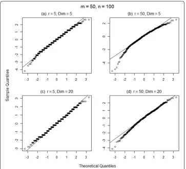
Simulation suggests that the null distribution ofTris negatively skewed, but that for
sufficiently largeNand possibly certain conditions onrthis distribution is asymptotic-ally normal, independent of distribution function F. Rosenbaum (2005) proves that Tr
is asymptotically normal forr= 1 for any distribution function; proof of this conjecture for r> 1 remains an open problem. This conjecture is supported by the normal
QQ-plots shown in Figures 3 and 4 for 1,000 simulated values of ðTr−E T½ rÞ=
ffiffiffiffiffiffiffiffiffiffiffiffiffiffiffiffiffi
Varð ÞTr p
at r= 5, 50 andN= 150, 600 withm/n= 1/2, under sampling from uniform distributions on [−1, 1]5 and [−1, 1]20. For the smaller sample size (N= 150), negative skewness is stronger for lower dimension and for higherr, withr= 50 and Dim = 5 being the most strongly skewed case shown. For the larger sample size (N= 600), skewness effects ap-pear to vanish for all but ther= 50 and Dim = 5 case, and even in this case skewness is vastly diminished compared to the smaller sample size. Other distribution families and other values ofm/nproduce similar results.
Figure 4Normal QQ-plots of 1,000 simulated values ofTrform= 200, n= 400 andr= 5, 50.Panels (a)and(b)are from independent samples of Unif [−1, 1]5variates. Panels(c)and(d)are from independent samples of Unif [−1, 1]20variates.
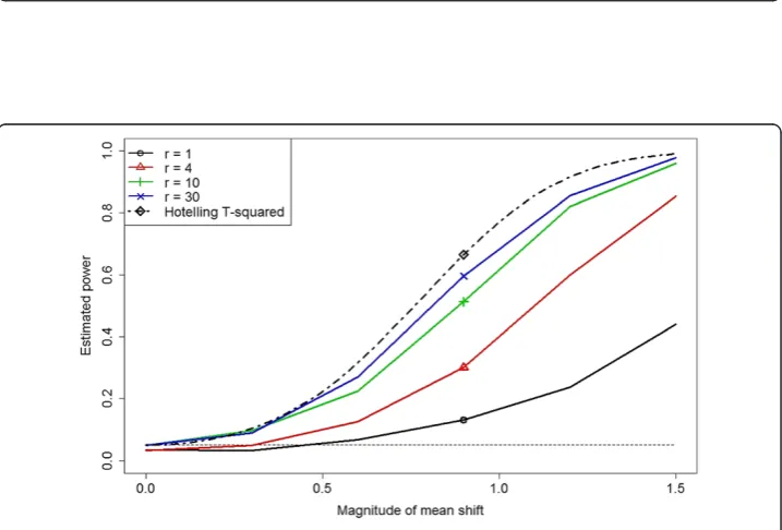
Figure 5Power estimates for the MCC test atr= 1, 4, 10, and 30 and exact power for Hotelling’sT2
Future work remains to bound rejection region probabilities in terms of sample size, dimension, and choice ofr. In the absence of such theoretical bounds, for practical pur-poses a permutation test on observation indices serves as a suitable method to estimate p-values for the MCC test in cases where a normal approximation cannot be justified.
3.2 Small simulation study
We compare power characteristics of tests for two different location-shift scenarios. For each case, 1000 simulations are conducted for each shift in location parameter, group sizes are m= 20 andn= 40, and tests are conducted at significance levelα= .05. Distances are Euclidean. Estimated power is shown for MCC tests withr= 1, 4, 10, and 30 (where r= 1 is the cross-match test), and the performance of these tests is compared directly to that of Hotelling’sT2test. Critical values for the MCC test were estimated through simulation for this study. All simulations were performed in R.
For the first example, the smaller group is drawn from a multivariate normal distribu-tion with mean vector0, identity covariance matrix, and dimension 5. The larger group is drawn from the same family, but the location vector of the second group isΔ, where
Δ ranges in magnitude from 0 to 1.5 by increments of 0.3. Hotelling’sT2test is known to be the uniformly most powerful invariant test for location shift under these condi-tions (Bilodeau and Brenner 1999) and the exact power of the test is known for all loca-tion alternatives.
Figure 5 displays the estimated power results. We notice immediately that a modest increase ofr= 1 tor= 4 substantially improves on the power of the cross-count test. As r continues to increase, MCC performance is even more impressive; the r= 30 =N/2 case performs nearly as well as Hotelling’sT2test. Power estimates for casesr>N/2 are not shown. Not surprisingly, test power generally decreases as rincreases beyondN/2 towardN−1; in the extreme caseTN−1takes the fixed value Nmn−1 and hence the MCC test withr=N−1 has power equal to zero against all alternatives.
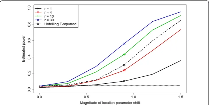
Figure 6Power estimates for the MCC test atr= 1, 4, 10, and 30 and estimated power for Hotelling’sT2statistic for 5-variate lognormal location parameter alternatives withm= 20 and
For the second example, the first group is drawn from the multivariate log-normal distribution, where each of the 5 dimensions consists of independent, univariate log-normal draws with location parameter 0 and scale parameter 1. As before, the second group is drawn from the same family, but the location parameter vector for the second group is Δ, where the magnitude of Δ ranges from 0 to 1.5 by increments of 0.3 and each dimension of Δ takes equal value. The lognormal distribution is considered here to examine the effects of a skewed distribution on the tests in question. Since the underlying distributions are no longer multivariate normal, the power of Hotelling’sT2 test is estimated by simulation for this example.
Figure 6 displays the estimated power results. As before, we see that the power of the MCC test with r= 4 is much better than forr= 1. It is particularly noteworthy that for sufficiently largerthe MCC test outperforms Hotelling’sT2test.
4 Conclusions
The mean cross-count test is a powerful, non-parametric multivariate two-sample test that is applicable to any case where a notion of distance between observations exists. While this paper considers only location shifts, other simulations show that the MCC test has power in a variety of alternative cases as well. A shortcoming of the MCC test is that the null distribution forTr is not simple (and perhaps not possible) to compute
for all r> 1 and is not exactly distribution-free in these cases; in contrast, the test upon which it is based, the cross-match test withr= 1, has a known distribution that is inde-pendent of the distribution being tested.
It is known that T1is asymptotically normal, and while the mean and variance ofTr
are derived herein and simulation suggests that the normal approximation forTris
ap-propriate for sufficiently large N with r> 1, this property remains to be proven. This proof is part of ongoing work, as is sharpening the normal approximation via Edge-worth expansion based on higher moments of Tr. Likewise, finding useful criteria for
choosingris another area for future work.This choice is subject to competing factors: On the one hand, the power ofTrappears to improve asrincreases toN/2 when group
sizes are equal (i.e., m=n=N/2); therefore, r=N/2 seems a good choice for equal group sizes. On the other hand, the normal approximation appears to worsen as r in-creases; thus it may be desirable to restrict the size ofrfor this sake. Furthermore, an additional effect exists when group sizes are different. For example, assume m<n. If r≥m, then at least one edge in Gr contains a vertex from each group and contributes to the cross-count, increasing the value of Tr. This is true even if the two groups are
very different. Since a higher cross-count weakens the evidence against a group differ-ence, this consideration suggests choosing r< min(m,n). A similar effect exists for multimodal distributions, suggesting that the size ofrmight be restricted as the num-ber of modes grows. In any case, the best choice of rin practice clearly depends upon application specifics.
Competing interest
The author declares that he has no competing interests.
References
Anderson, I: Perfect matchings of a graph sufficient conditions for matchings. Proc Edinburgh Math Soc18, 129–136 (1972). Ser. 2
Bilodeau, M, Brenner, D: Theory of Multivariate Statistics. Springer, New York (1999)
Friedman, J, Rafsky, L: Multivariate generalizations of the Wald-Wolfowitz and Smirnov two-sample tests. Ann Stat 7, 697–717 (1979)
Friedman, J, Rafsky, L: Graphics for the multivariate two-sample problem. JASA76, 277–287 (1981)
Hall, P, Tajvidi, N: Permutation tests for equality of distributions in high-dimensional settings. Biometrika89, 359–374 (2002)
Henze, N: A multivariate two-sample test based on the number of nearest neighbor type coincidences. Ann Stat 16, 772–783 (1988)
Maa, J, Pearl, D, Bartoszynski, R: Reducing multidimensional two-sample data to one-dimensional interpoint comparisons. Ann Stat24, 1069–1074 (1996)
Rosenbaum, P: An exact distribution-free test comparing two multivariate distributions based on adjacency. JRSS B 67, 515–530 (2005)
Ruth, D, Koyak, K: Nonparametric tests for homogeneity based on non-bipartite matching. JASA106, 1615–1625 (2011) Schilling, M: Multivariate two-sample tests based on nearest neighbors. JASA81, 799–806 (1986)
doi:10.1186/s40488-014-0022-4
Cite this article as:Ruth:A new multivariate two-sample test using regular minimum-weight spanning subgraphs.Journal of Statistical Distributions and Applications20141:22.
Submit your manuscript to a
journal and benefi t from:
7 Convenient online submission
7 Rigorous peer review
7 Immediate publication on acceptance
7 Open access: articles freely available online 7 High visibility within the fi eld
7 Retaining the copyright to your article