The generalized Cauchy family of distributions with applications

M E T H O D O L O G Y

Open Access

The generalized Cauchy family of

distributions with applications

Ayman Alzaatreh

, Carl Lee

, Felix Famoye

and Indranil Ghosh

* Correspondence:

ayman.alzaatreh@nu.edu.kz 1_{Department of Mathematics,}

Nazarbayev University, Astana, KZ 010000, Kazakhstan

Full list of author information is available at the end of the article

Abstract

A family of generalized Cauchy distributions,T-Cauchy{Y} family, is proposed using theT-R{Y} framework. The family of distributions is generated using the quantile functions of uniform, exponential, log-logistic, logistic, extreme value, and Fréchet distributions. Several general properties of theT-Cauchy{Y} family are studied in detail including moments, mean deviations and Shannon’s entropy. Some members of the

T-Cauchy{Y} family are developed and one member, gamma-Cauchy{exponential} distribution, is studied in detail. The distributions in theT-Cauchy{Y} family are very flexible due to their various shapes. The distributions can be symmetric, skewed to the right or skewed to the left.

Keywords:T-R{Y} framework, Quantile function, Moments, Shannon’s entropy

1. Introduction

The Cauchy distribution, named after Augustin Cauchy, is a simple family of dis-tributions for which the expected value does not exist. Also, the family is closed under the formation of sums of independent random variables, and hence is an in-finitely divisible family of distributions. The Cauchy distribution was used by Stigler (1989) to obtain an explicit expression for P(Z1≤0,Z2≤0) where (Z1,Z2)T

follows the standard bivariate normal distribution. The Cauchy distribution has been used in many applications such as mechanical and electrical theory, physical anthropology, measurement problems, risk and financial analysis. It was also used to model the points of impact of a fixed straight line of particles emitted from a point source (Johnson et al. 1994). In Physics, it is called a Lorenzian distribution, where it is the distribution of the energy of an unstable state in quantum mechanics.

Eugene et al. (2002) introduced the beta-generated family of distributions using the beta as the baseline distribution. Based on the beta-generated family, Alshawarbeh et al. (2013) proposed the beta-Cauchy distribution. The beta-generated family was extended by Alzaatreh et al. (2013) to theT-R(W) family. The cumulative distribution

function (CDF) of the T-R(W) distribution is G xð Þ ¼

∫

a r tð Þdt; where r(t) is the probability density function (PDF) of a random variable T with support (a, b) for − ∞ ≤a<b≤ ∞. The link function W: [0, 1]→ ℝ is monotonic and absolutely continuous with W(0)→a and W(1)→b.

Aljarrah et al. (2014) considered the function W(.) to be the quantile function of a random variable Y and defined the T-R{Y} family. In the T-R{Y} framework, the random variable T is a ‘transformer’ that is used to ‘transform’ the random variable R into a new family of generalized distributions of R. Many families of generalized distributions have appeared in the literature. Alzaatreh et al. (2014, 2015) studied the T-gamma and the T-normal families. Almheidat et al. (2015) studied the T -Weibull family. In this paper, a family of generalized Cauchy distribution is pro-posed and studied.

This article focuses on the generalization of the Cauchy distribution and studies some new distributions and their applications. The article gives a brief review of the T-R{Y} framework and defines several new generalized Cauchy sub-families. It contains some general properties of theT-Cauchy{Y} distributions. A member of the T-Cauchy{Y} family, the gamma-Cauchy{exponential} distribution, is studied. The study includes moments, estimation and applications. Some concluding remarks were provided.

2. The T-Cauchy{Y} family of distributions

The T-R{Y} framework defined in Aljarrah et al. (2014) (see also Alzaatreh et al. 2014) is given as follows. Let T, R and Y be random variables with CDF FZ(x) = P(Z≤x), and corresponding quantile function QZ(p), where Z=T, R, Y and the

quantile function is defined as QZ(p) = inf{z:FZ(z)≥p}, 0 <p< 1. If densities exist,

we denote them by fZ(x), for Z=T, R and Y. Now assume the random variables T,Y∈(a,b) for − ∞ ≤a<b≤ ∞. The random variable X in T-R{Y} family of distribu-tions is defined as

FXð Þ ¼x

∫

ð Þ

ð Þ

a fTð Þt dt¼FTðQYðFRð Þx ÞÞ: ð1Þ

The corresponding PDF associated with (1) is

f_Xð Þ ¼x f_TðQ_YðFRð ÞxÞÞ Q′YðFRð Þx Þ fRð Þx: ð2Þ

Alternatively, (2) can be written as

f_Xð Þ ¼x f_Rð Þ x fTðQYðFRð ÞxÞÞ f_YðQYðFRð ÞxÞÞ

: ð3Þ

The hazard function of the random variableXcan be written as

hXð Þ ¼x hRð Þ x hTðQYðFRð Þx ÞÞ hYðQYðFRð Þx ÞÞ

: ð4Þ

Let R be a random variable that follows the Cauchy distribution with PDF fR(x) = fC(x) =π−1θ−1(1 + (x/θ)2)−1 and CDF FR(x) =FC(x) = 0.5 +π−1tan−1(x/θ), x∈ℝ, θ> 0,

then (3) reduces to

f_Xð Þ ¼x f_Cð Þ x fTðQYðFCð Þx ÞÞ f_YðQYðFCð Þx ÞÞ

: ð5Þ

Hereafter, the family of distributions in (5) will be called the T-Cauchy{Y} family. It is clear that the PDF in (5) is a generalization of Cauchy distribution. From (1),

if T¼dY; then X¼dCauchyð Þ:θ Also, if Y¼dCauchyð Þ;θ then X¼dT: Furthermore, when T~ beta(a,b) and Y~ uniform(0, 1), the T-Cauchy{Y} reduces to the beta-Cauchy distribution (Alshawarbeh et al. 2013). WhenT~ Power(a) andY~ uniform(0, 1), theT-Cauchy{Y} reduces to the exponentiated-Cauchy distribution (Sarabia and Castillo 2005). Table 1 gives six quantile functions of known distributions (in standard form) which will be applied to generateT-Cauchy{Y} sub-families in the following subsections. It is straightforward to use non-standard quantile functions. By using non-standard quan-tile functions, many resulting distributions in theT-R{Y} family will have more than five parameters, which are not practically useful (Johnson et al. 1994, p. 12). Thus, we focus on the standard quantile functions in this paper.

2.1 T-Cauchy{uniform} family of distributions

By using the quantile function of the uniform distribution in Table 1, the corresponding CDF to (1) is

FXð Þ ¼x FTfFCð Þxg; ð6Þ

and the corresponding PDF to (6) is

f_Xð Þ ¼x f_Cð Þ x f_TðFCð ÞxÞ; x∈ℝ: ð7Þ

2.2 T-Cauchy{exponential} family of distributions

By using the quantile function of the exponential distribution in Table 1, the corre-sponding CDF to (1) is

FXð Þ ¼x FTf−log 1ð −FCð Þx Þg ð8Þ

and the corresponding PDF to (8) is

f_Xð Þ ¼x fCð Þx

1−Fcð Þx fTð−log 1ð −Fcð ÞxÞÞ; x∈ℝ: ð9Þ

Table 1Quantile functions for differentYdistributions

Y QY(p)

(a) Uniform p

(b) Exponential −log(1−p)

(c) Log-logistic p/ (1−p)

(d) Logistic log[p/(1−p)]

(e) Extreme value log[−log(1−p)]

Note that the CDF and the PDF in (8) and (9) can be written as FX(x) = FT(HC(x)) and fX(x) =hC(x)fT(HC(x)) where hC(x) and HC(x) are the hazard and

cu-mulative hazard functions for the Cauchy distribution, respectively. Therefore, the T-Cauchy{exponential} family of distributions arises from the ‘hazard function of the Cauchy distribution’.

2.3 T-Cauchy{log-logistic} family of distributions

By using the quantile function of the log-logistic distribution in Table 1, the corre-sponding CDF to (1) is

FXð Þ ¼x FTfFCð Þx=½1−FCð Þxg; ð10Þ

and the corresponding PDF is

f_Xð Þ ¼x fCð Þx

1−FCð Þx

ð Þ2fT

FCð Þx

1−FCð Þx

; x∈ℝ: ð11Þ

which is a family of generalized Cauchy distributions arising from the ‘odds’ of the Cauchy distribution.

2.4 T-Cauchy{logistic} family of distributions

By using the quantile function of the logistic distribution in Table 1, the corresponding CDF to (1) is

FXð Þ ¼x FTflogðFCð Þx =½1−FCð Þx Þg; ð12Þ

and the corresponding PDF is

f_Xð Þ ¼x fCð Þx

FCð Þx½1−FCð Þx fTðlogðFCð Þx =½1−FCð Þx ÞÞ; x∈ℝ: ð13Þ

Note that (13) can be written as f_Xð Þ ¼x hCð Þx

FCð Þx fT log

FCð Þx 1−FCð Þx

, which is a family

of generalized Cauchy distributions arising from the ‘logit function’ of the Cauchy distribution.

2.5 T-Cauchy{extreme value} family of distributions

By using the quantile function of the extreme value distribution in Table 1, the corre-sponding CDF to (1) is

FXð Þ ¼x FTflogð−log 1½ −FCð Þx Þg; ð14Þ

and the corresponding PDF is

f_Xð Þ ¼x fCð Þx FCð Þx−1

½ log 1ð −FCð ÞxÞfTflog½−log 1ð −FCð ÞxÞg; x∈ℝ: ð15Þ

2.6 T-Cauchy{Fréchet} family of distributions

By using the quantile function of the Fréchet distribution in Table 1, the corresponding CDF to (1) is

FXð Þ ¼x FTf−1=logðFCð ÞxÞg; ð16Þ

and the corresponding PDF is

f_Xð Þ ¼x fCð Þx FCð ÞxðlogFCð Þx Þ2

f_Tf−1=logðFCð Þx Þg; x∈ℝ: ð17Þ

Figures 1 and 2 show some examples of two members of the T-Cauchy{Y} family. The first example is Weibull-Cauchy{exponential} distribution which can be obtained by replacing the random variable T in (9) with Weibull(c,γ) random variable. The second example is Lomax-Cauchy{log-logistic} distribution which can be obtained by replacing the random variable T in (11) with Lomax(α,λ) random variable. From the figures, it appears that the shapes of the distributions can be left-skewed, right-skewed or symmetric.

3. Some properties of the T-Cauchy{Y} family of distributions

In this section, we discuss some general properties of the T-Cauchy family of distribu-tions. The proofs are omitted for straightforward results.

Lemma 1: LetTbe a random variable with PDFfT(x), then

(i) The random variableX=−θcot(πF_Y(T)) follows theT-Cauchy{Y} distribution. (ii)The quantile function forT-Cauchy{Y} family isQX(p) =−θcot(πFY(QT(p))).

The Shannon’s entropy (Shannon 1948) of a random variable X is a measure of variation of uncertainty and it is defined as ηX=−E{log(f(X))}. The following

prop-osition provides an expression for the Shannon’s entropy for the T-Cauchy{Y} family.

Proposition 1: The Shannon’s entropy for theT-Cauchy{Y} family is given by

ηX ¼ logð Þθ−logð Þ þπ ηTþEðlogfYð ÞT Þ−2EflogðFYð ÞT Þg−2

X∞

j¼1

VjE F½ Yð ÞT 2j: ð18Þ

Proof: By using the result in Aljarrah et al. (2014), the Shannon’s entropy for the T-Cauchy{Y} is

ηX¼ηTþEðlogfYð ÞT Þ−EflogfCðQCðFYð ÞT ÞÞg: ð19Þ

Now, one can show that

logf_CðQCðFYð Þt ÞÞ ¼−logð Þ þπθ 2 log sinð ðπFYð Þt ÞÞ: ð20Þ

On using the following series expansion from Gradshteyn and Ryzhik (2007, p. 55)

log sinð ð Þπx Þ ¼ logð Þ þπx X

∞

j¼1

Vjx2j; ð21Þ

whereVj¼ð Þ−1jð Þ2π2jB2j

2jð Þ2j! andBjis the Bernoulli number, we get the result in (18). □ Next proposition gives a general expression for the r-th moment for theT-Cauchy{Y} family.

Proposition 2: Ther-th moment for theT-Cauchy{Y} family of distributions is given by

E Xð Þ ¼r ð Þ−1 rθrX ∞

k¼0

ckE FY½ ð ÞT 2k−r; ð22Þ

wherec0=π−r,cm¼πm−1

X k¼1

m

kr−mþk

ð Þwkcm−k; m≥1 andwk ¼ð Þ−1 k

22k_B

2kπ2k−1

2k

ð Þ! :

Proof: From Lemma 1(i), the r-th moment for the T-Cauchy{Y} family can be written as E(Xr) = (−1)rθrE(cotπ(FY(T)))r. Now, using the following series

expan-sion (see Abramowitz and Stegun 1964, p.75), cotðπxÞ ¼X ∞

k¼0

wkx2k−1;jxj<π;

where wk¼ð Þ−1

k 22k_B

2kπ2k−1 2k

ð Þ! :Therefore,

cotπðFYð Þt Þ

ð Þr_¼X∞

k¼0

ckðFYð Þt Þ2k−r; ð23Þ

where c0=π−r, cm¼πm−1

Xm

k¼1

kr−mþk

ð Þwkcm−k; m≥1 [see Gradshteyn and Ryzhik

2007, p. 17]. □

As an example of the applicability of the results in Lemma 1 and Propositions 1 and 2, we use these results and apply them on the T-Cauchy{exponential}. One can get similar results by choosing any of theT-Cauchy{Y} families.

Corollary 1: Based on Lemma 1, ifTis a random variable with PDFfT(x), then

(i) The random variable X=θcot(πe−T) follows a distribution in the T-Cauchy{exponential} family.

(ii)The quantile functions forT-Cauchy{exponential} family isQXð Þ ¼p θcotπe−QTð Þp:

Corollary 2: The Shannon’s entropy for the T-Cauchy{exponential} family is given by

ηX¼ logð Þθ −logð Þ þπ ηTþμT−2 X∞

j¼1

VjMTð−2jÞ;

whereMT(.) is the moment generating function of the random variableT.

Proof:The result follows from Proposition 1 and the fact thatE(logfY(T)) =μT. □ Corollary 3: The r-th moment for theT-Cauchy{exponential} family of distributions is given by

E Xð Þ ¼r θrX

∞

k¼0

ckMTðr−2kÞ;

whereckis defined in Proposition 2.

Proof: The result follows from Proposition 2 and the fact that cot(πFY(u)) =−cot(πe−u). □ Proposition 3: The mode(s) of theT-Cauchy{exponential} family are the solutions of the equation

x¼ θ

2πhCð Þx 1þ

f′_TðHCð Þx Þ f_TðHCð Þx Þ ( )

: ð24Þ

Proof: For Cauchy distribution, one can show that f′_Cð Þ ¼x −2πθ−1x f2_Cð Þx and

h′_Cð Þ ¼x −2πθ−1xhCð Þ þx h2Cð Þ:x On findingf′Xð Þx by using Eq. (9) and setting the deriva-tive to zero, it is easy to get the result in (24). □

4. Gamma-Cauchy{exponential} distribution

For the remaining sections, we investigate in details the properties, parameter estima-tion and applicaestima-tions of a new distribuestima-tion of the T-Cauchy{Y} family, the gamma-Cauchy{exponential} distribution. This distribution is interesting as it consists of special cases of exponentiated Cauchy and distributions of record values from the Cauchy dis-tribution. LetTbe a random variable that follows the gamma distribution with parame-ters α andβ. From Eqs. (8) and (9), the PDF and CDF of gamma-Cauchy{exponential} distribution are, respectively, given by

f xð Þ ¼ −log 0:5−π

−1_tan−1_ðx=θÞ

ð Þ

½ α−1

0:5−π−1_tan−1_ðx=θÞ

½ 1β−1

πθβα_{Γ αð Þ1þðx=θÞ}2 ; x∈ℝ; ð25Þ

F xð Þ ¼γ α;−β

−1_{log 0ð :5−π}−1_tan−1_ðx=θÞÞ

whereγ α;ð xÞ ¼

∫

0tα−1e−tdtis the incomplete gamma function. For simplicity, a random variableXwith PDFf(x) in (25) is said to follow the gamma-Cauchy{exponential} distri-bution and is denoted byGC(α,β,θ).

Some special cases are worth mentioning:

(i) GC(1,β,θ) is the exponentiated Cauchy distribution proposed by Sarabia and Castillo (2005). In particularGC(1,1,1) is the standard Cauchy distribution. (ii) GC(1,n−1,θ),n∈ℕis the distribution of the minimum ofnindependent Cauchy

random variables.

(iii)GC(n+ 1, 1,θ),n∈ℕis the distribution of thenth upper record in a sequence of independent Cauchy random variables.

Remarks:The following results follow from Corollary 1, Corollary 2 and Proposition 3.

(i) If a random variableYfollows a gamma distribution with parametersαandβ, then

X=θcot(πe−Y) follows theGC(α,β,θ) distribution.

(ii) The quantile function ofGC(α,β,θ) isQ pð Þ ¼θcot πe−βγ−1½α;pΓ αð Þ

; 0<p<1: (iii) The Shannon’s entropy for theGC(α,β,θ) distribution is given by

ηX¼αð1þβÞ þ logðπ−1θβΓ αð ÞÞ þð1−αÞψ αð Þ−2 X∞

j¼1

Vjð1þ2jβÞ−α; where ψ(.) is the

digamma function andVjis defined in Eq. (21).

Proposition 4: The GC(α,β,θ) distribution is unimodal and the mode is at m=θx wherexis the solution of the equation

k xð Þ ¼ log cot −1_{ð Þx}

π

2xcot−1ð Þx −1þ1=β

þα−1¼0:

Proof: It is not difficult to show that the mode of f(x) in (25) is the solution of k(x/θ) = 0, where k(x) is defined above. Therefore, the mode of f(x) is at m=θx where k(x) = 0. To show the unimodality of f(x), consider A(x) = log(π−1cot−1(x)) and B(x) = 2xcot−1(x). Clearly A(x) is a strictly decreasing function (since it is equal to log(1−FC(x))). Furthermore, A(x) < 0 for all x∈ℝ. Now, B′(x) = 2[−x/(1 + x2) + cot−1(x)]. Therefore, B′(x) > 0 for all x≤0. If x> 0, we have B′(x) <B′(0) =π/2 since B″(x) < 0. Since lim

x→∞ B

′_{ð Þ ¼x 0: we get B′(x) > 0 for all x> 0. Therefore, B(x) is}

strictly increasing for all x∈ℝ. Now, let us prove the claim that η(x) =A(x)B(x) is a decreasing function on ℝ.

Proof of the claim: Let 0≤x≤y, then 0≤ −A(x)≤ −A(y) and 0≤B(x)≤B(y). This implies that η(x)≥η(y). Now let x< 0, then η′(x) =−2x/(x2+ 1)−2(x2+ 1)−1x log(π−1cot−1(x)) + 2 cot−1(x)log(π−1cot−1(x)). Since the middle term inη′(x) is negative,

consider ψð Þ ¼x x

x2_þ1−cot−1ð Þx log cotð −1ð Þ=x πÞ: On differentiation, ψ′ð Þ ¼x _x21_þ1

2

x2_þ1þ log cotð −1ð Þ=x πÞ

n o

: It is easy to show that the term ζð Þ ¼x _x22_þ1þ log

cot−1_{ð Þ=x π}

Hence, η(x) =A(x)B(x) is a decreasing function in ℝ. This completes the proof of the claim. The fact thatη(−∞)→2 andη(∞)→− ∞implies thatη(x) = 0 has a unique so-lution. Now, B(x)−1 + 1/β is only a shift by −1 + 1/β and therefore remains a strictly increasing function. One can show that the termA(x)[B(x)−1 + 1/β] remains a de-creasing function for all x∈ℝ and hence k(x) remains a decreasing function in ℝ with k(−∞)→α+ 1 > 0 andk(∞)→− ∞. This ends the proof. □

In Fig. 3, various graphs off(x) are provided for different parameter values ofαandβ where θ= 1. The plots indicate that the gamma-Cauchy{exponential} distribution can be symmetric, right-skewed or left-skewed. Also, it appears that gamma-Cauchy{exponential} is symmetric only for the trivial case when α=β= 1.

In the following subsection, we provide some results related to the moments of GC(α,β,θ) distribution.

4.1 Moments of gamma-Cauchy{exponential} distribution

From Corollary 3, ther-th moment of theGC(α,β,θ) can be written as

μ′

rðα;β;θÞ ¼E Xð Þ ¼r θr X∞

k¼0

ck½1−βðr−2kÞ−α; ð27Þ

whereckis defined in Eq. (22). Therefore, the mean ofGC(α,β,θ) is

μ′

1ðα;β;θÞ ¼θ

X∞

k¼0

ck½1−βð1−2kÞ−α;

whereckis defined in (22) with r= 1. Note thatμ′1ðα;β;θÞis defined here forα> 1 and

β< 1.

The next proposition establishes the condition for the existence of r-th moment of theGC(α,β,θ) distribution.

Proposition 5: The r-th moment of the GC(α,β,θ) distribution exists if and only if α>randβ−1>r.

Proof: Without loss of generality, we assume θ= 1 and apply a similar idea as in Alshawarbeh et al. (2012). We write

E Xð Þ ¼r

∫

1

−∞xrg xð Þdxþ

∫

−1xrg xð Þdxþ

∫

1xrg xð Þdx: ð28Þ

Since the middle integrand is bounded by 2, it suffices to investigate the existence of the

first and third integrands of the right hand side of Eq. (28). ConsiderI1¼

∫

∞

1xrg xð Þdxand

I2¼

∫

−1

−∞xrg xð Þdx:Consider the following inequality from Abramowitz and Stegun (1964), p. 68

x<−log 1ð −xÞ< x

1−x; x<1; x≠0: ð29Þ

On using the inequality in (29) and forα> 1, we have

I1≤ 1 πβα_{Γ αð Þ}

∫

∞ 1

xr

1þx2 1=2þπ

−1_tan−1_{ð Þx}

α−1

1=2−π−1tan−1ð Þx 1=β−α

dx:

Let us write δð Þ ¼x xr

1þx2ð1=2þπ−1tan−1ð ÞxÞ

α−1 _1=2−π−1

tan−1_{ð Þx}

ð Þ1=β−α. Then one can show that asx→∞,δ(x) ~x−(1/β−α−r+ 2). Therefore,I1exists if and only if 1/β−α>r−1.

Sinceα> 1, this implies 1/β>r. Now, ifα< 1, the inequality in (29) implies that

I1≤ 1 πβα_{Γ αð Þ}

∫

∞ 1

xr

1þx2 1=2þπ

−1_tan−1_{ð Þx}

α−1

1=2−π−1tan−1ð Þx 1=β−1

:

Letζð Þ ¼x xr

1þx2ð1=2þπ−1tan−1ð Þx Þ α−1

1=2−π−1_tan−1_{ð Þx}

ð Þ1=β−1_:

Asx→∞,ζ(x) ~x−(1/β−r+ 1). SoI1exists if and only if 1/β>r. Similarly one can show thatI2exists if and only ifα>r. □

Next, we consider recursive relation for the r-th moment of the GC(α,β,θ) distribution.

Proposition 6: LetX~GC(α,β, 1) andn∈ℕ. Then

(i)μ′_2nðα;βÞ ¼ 1

πβð1−βÞα−1 Xn

j¼1 −1 ð Þj−1 2n−2jþ1 μ

′

2n−2jþ1 α;1−ββ

−μ′

2n−2jþ1 α−1;1−ββ

n o

þð Þ−1 n:

(ii)μ2nþ1′ðα;βÞ ¼_πβð1−1βÞα−1

Xn

j¼1 Xj

i¼0 −1 ð Þn−j

2j

n

j ji μ′2i α;1β−β

−μ′

2i α−1; 1β−β

n o

þð Þ−1nμ′_ðα;βÞ:

Proof:From (25) and using the substitutionu=tan−1(x), we have

πβα_{Γ αð Þμ}′ 2n¼

∫

π=2 −π=2ðtanuÞ

2n

−log 0 :5−π−1u α−1

0:5−π−1u 1=β−1

du¼X n

j¼0

Ij; ð30Þ

where

I0¼ð Þ−1 n

∫

π=2

−π=2 −log 0:5−π−1u

α−1

0:5−π−1u 1=β−1

du

and

Ij¼ð Þ−1 j−1

∫

−π=2tan2n−2jð Þu sec2ð Þu −log 0:5−π−1u

α−1

0:5−π−1u 1=β−1

du; j≥1:

It is easy to see thatI0= (−1)nπβαΓ(α). Also, it is not difficult to show that

Ij¼ð Þ−1 j−1_{Γ αð Þ}

2n−2jþ1 β 1−β

α−1

μ′

2n−2jþ1 α;

β 1−β

−μ′

2n−2iþ1 α−1;

β 1−β

Substituting (31) in (30), we get the result in (i). For the proof of (ii), one can easily see that

πβα_{Γ αð Þμ}′

2nþ1¼ð Þ−1

n_{π β}α_{Γ αð Þμ}′_{ðα;βÞ þ}Xn

j¼1

Ij;

where

Ij¼ð Þ−1 n−j n

j

∫

π=2

−π=2sec2j−1ð Þu secutanu −log 0:5−π−1u

α−1

0:5−π−1u 1=β−1

du:

The rest of the proof is not difficult to show. □

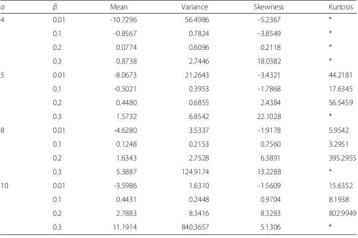
Table 2 provides the mean, variance, skewness and kurtosis of theGC(α,β, 1) for vari-ous values of α and β. For fixed α, the mean and skewness are increasing functions of β. Also, for fixedβ, the mean is an increasing function ofα. Furthermore, the values of the skewness from Table 2 show that the distribution is very flexible in terms of shapes and the distribution can be left or right skewed.

Skewness and kurtosis of a distribution can be measured byβ1=μ3/σ3andβ2=μ4/σ4,

respectively. However, the third and fourth moments ofGC(α,β,θ) do not always exist (see Proposition 5). Alternatively, we can define the measure of asymmetry and tail weight based on quantile function. The Galton’s skewness S defined by Galton (1883) and the Moors’kurtosisKdefined by Moors (1988) are given by

S¼Qð6=8Þ−2Qð4=8Þ þQð2=4Þ

Qð6=8Þ−Qð2=8Þ : ð32Þ

K¼Qð7=8Þ−Qð5=8Þ þQð3=8Þ−Qð1=8Þ

Qð6=8Þ−Qð2=8Þ : ð33Þ

Table 2Mean, variance, skewness and kurtosis calculations forGC(α,β,1)

α β Mean Variance Skewness Kurtosis

4 0.01 -10.7296 56.4986 -5.2367 *

0.1 -0.8567 0.7824 -3.8549 *

0.2 0.0774 0.6096 0.2118 *

0.3 0.8738 2.7446 18.0382 *

5 0.01 -8.0673 21.2643 -3.4321 44.2181

0.1 -0.5021 0.3953 -1.7868 17.6345

0.2 0.4480 0.6855 2.4384 56.5459

0.3 1.5732 6.8542 22.1028 *

8 0.01 -4.6280 3.5337 -1.9178 5.9542

0.1 0.1248 0.2153 0.7560 3.2951

0.2 1.6343 2.7528 6.3891 395.2955

0.3 5.3887 124.9174 13.2288 *

10 0.01 -3.5986 1.6310 -1.5609 15.6352

0.1 0.4431 0.2448 0.9704 8.1938

0.2 2.7883 8.3416 8.3283 802.9949

0.3 11.1914 840.3657 5.1306 *

When the distribution is symmetric,S= 0 and when the distribution is right (or left) skewed S> 0 (or S< 0). AsKincreases the tail of the distribution becomes heavier. To investigate the effect of the two shape parameters α and βon the GC(α,β,θ) distribu-tion, Eqs. (32) and (33) are used to obtain the Galtons’skewness and Moors’ kurtosis where the quantile function is defined in Remark (ii). Figure 4 displays the Galton’s skewness and Moors’ kurtosis for the GC(α,β, 1). From this figure, it appears that the GC(α,β,θ) distribution has a wide range of skewness and kurtosis. It can be left skewed, right skewed or symmetric.

4.2 Estimation of parameters by maximum likelihood method

Let X1,X2,…,Xn be a random sample of size n drawn from the GC(α,β,θ). The

log-likelihood function is given by

ℓ¼−nlogðπθΓð ÞαβαÞ−log 1ð þðxi=θÞÞ þ β−1−1

Xn

i¼1

logð Þ þzi ðα−1Þ

Xn

i¼1

logð−logð Þzi Þ;

ð34Þ

wherezi= 0.5−π−1tan−1(xi/θ).

The derivatives of (34) with respect toα,βandθare given by

∂ℓ

∂α¼−nψ αð Þ−nlogβþ Xn

i¼1

logð−logð Þzi Þ; ð35Þ

∂ℓ

∂β¼−

nα

β þ 1 β2

Xn

i¼1

logð Þzi ; ð36Þ

∂ℓ

∂θ¼−

n

θþ Xn

i¼1

xi

θ θð þxiÞ

þXn

i¼1

xi

π θ2_þx2

i

zi ðα−1Þðlogð Þzi Þ

−1_þ

1=β−1

; ð37Þ

whereψ(α) =∂logΓ(α)/∂α, is the digamma function.

Therefore, the MLEα^;β^ andθare obtained by setting the Eqs. (35), (36) and (37) to zero and solving them simultaneously. Note that the number of equations can be

re-duced to two by using Eq. (36) to get β¼X n

i¼1

logð Þzi

nα : The initial value for the

parameter θ can be taken as θ0= 1. From Remark (i) in Gamma-Cauchy{exponential}

distribution, the random variableYi=−log[0.5−π−1tan−1(Xi/θ0)],i= 1, 2,…,nfollows

a gamma distribution with parameters α and β. Therefore, by equating the sample mean and sample variance of Yiwith the corresponding population mean and variance,

the initial estimates forαand βare, respectively,α0¼y2=sy2 andβ0¼s2y=ywherey and

s2_y are the sample mean and sample variance foryi,i= 1,…,n.

4.3 Simulation study

A simulation study is conducted to evaluate the MLE in terms of estimates and stand-ard deviations for various parameter combinations and different sample sizes. We con-sider the values 0.5, 0.9, 1, 2, 5 for the parameterα, 0.5, 1, 3 for the parameterβ, and 1, 2 for the parameterθ. The simulation study for the MLE is conducted for a total of six parameter combinations and the process is repeated 200 times. Three different sample sizesn= 50, 100, 300 are considered. The ML estimates and the standard deviations are presented in Table 3. From this table, it appears that the ML estimates ofαandθtend to be overestimated. As expected, as the sample size increases, the bias and standard deviation values for all the estimates decrease.

4.4 Applications

In this section, the GC(α,β,θ) distribution is fitted to two data sets. The first data set from Bjerkedal (1960), represents the survival time in days of 72 guinea pigs infected with virulent tubercle bacilli. The first data set is

The data is skewed-to-the right with skewness = 1.3134 and kurtosis = 3.8509.

The second data set from Durbin and Koopman (2001), represents the measurements of the annual flow of the Nile River at Ashwan from 1871–1970. The second data set is

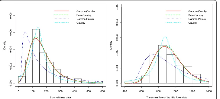
The data is approximately symmetric with skewness = 0.3175 and kurtosis = 2.6415. We fitted the two data sets to the GC(α,β,θ) distribution and compared the results with Cauchy, gamma-Pareto proposed by Alzaatreh et al. (2012) and beta-Cauchy distributions proposed by Alshawarbeh et al. (2013). The maximum likeli-hood estimates, the log-likelilikeli-hood value, the AIC (Akaike Information Criterion), the Kolmogorov- Smirnov (K-S) test statistic, and the p-value for the K-S statistic for the fitted distributions to the data sets 1 and 2 are reported in Tables 4 and 5 respectively.

The results in Tables 4 and 5 show the GC(α,β,θ) and beta-Cauchy provide an ad-equate fit to the survival time data while theGC(α,β,θ) distribution provides the best

10, 33, 44, 56, 59, 72, 74, 77, 92, 93, 96, 100, 100, 102, 105, 107, 107, 108, 108, 108, 109, 112, 121, 122, 122,124,130, 134, 136, 139, 144,146, 153, 159, 160, 163, 163,168, 171, 172, 176,113, 115, 116, 120, 183,195, 196, 197, 202, 213, 215, 216, 222, 230,231, 240, 245, 251, 253, 254, 255, 278, 293, 327, 342, 347, 361,402, 432, 458, 555

fit (based on KSp-value) to the annual flow of the Nile River data. The fact thatGC(α,β,θ) distribution has only three parameters compared with the beta-Cauchy distribution makes GC(α,β,θ) a natural choice for fitting these two data sets. A closer look at the parameter estimates for the beta-Cauchy distribution indicates that the estimates ofα,βandθin the beta-Cauchy distribution are not statistically significant for the two examples. This is an in-dication that beta-Cauchy is over-parameterized for fitting these two data sets. This sup-ports the point that the three-parameterGC(α,β,θ) distribution should be used to fit the two data sets. Figure 5 displays the histogram and the fitted density functions for the two data sets, which support the results in Tables 4 and 5.

Table 3Estimates and standard deviations for the parameters using MLE method

Sample size Actual values ML estimates Standard deviation

n α β θ ^α ^β ^θ ^α ^β ^θ

50 1 1 1 1.1605 0.9260 1.1455 0.0518 0.0460 0.0538

0.5 1 2 0.5377 0.9552 2.1399 0.0180 0.0426 0.0978

0.5 3 2 0.5351 2.8849 2.1952 0.0154 0.1207 0.1065

0.9 0.5 1 1.0229 0.4960 1.0579 0.0481 0.0222 0.0442

2 0.5 1 2.9571 0.4448 1.2255 0.4271 0.0282 0.0917

5 0.5 1 7.9697 0.4487 0.8862 0.9537 0.0183 0.0737

100 1 1 1 1.0717 0.9617 1.0499 0.0216 0.0230 0.0248

0.5 1 2 0.5182 1.0090 2.0843 0.0084 0.0229 0.0457

0.5 3 2 0.5165 2.9594 2.0505 0.0065 0.0591 0.0441

0.9 0.5 1 0.9375 0.4932 1.0309 0.0181 0.0105 0.0203

2 0.5 1 2.2258 0.4753 1.0866 0.0646 0.0131 0.0281

5 0.5 1 6.3436 0.4737 0.9243 0.4015 0.0089 0.0367

300 1 1 1 1.0244 0.9983 1.0270 0.0094 0.0114 0.0111

0.5 1 2 0.5076 0.9908 2.0320 0.0041 0.0102 0.0229

0.5 3 2 0.5113 2.9636 2.0718 0.0039 0.0315 0.0241

0.9 0.5 1 0.9242 0.4953 1.0159 0.0086 0.0053 0.0102

2 0.5 1 2.1286 0.4844 1.0369 0.0270 0.0071 0.0123

5 0.5 1 5.2815 0.4987 0.9562 0.1368 0.0040 0.0149

Table 4Parameter estimates for the survival time data

Distribution Cauchy Gamma-Pareto Beta-Cauchy Gamma-Cauchy{exponential}

Parameter

Estimates ĉ

= 139.3079 (9.4281)a ^

θ= 48.1262 (7.6793)

^

α= 6.030 (0.9770)

ĉ= 0.4497 (0.0760) ^

θ= 10

^

α= 13.9274 (18.5335) ^

β= 4.5828 (3.6504)

ĉ= 117.9055 (37.6269) ^

θ= 27.0884 (99.7681)

^

α= 16.1591 (2.6666) ^

β= 0.1027 (0.0238) ^

θ= 110.1742 (35.4345)

Log-likelihood -437.5967 -465.4670 -424.4339 -424.4423

AIC 879.1934 934.9340 856.8679 854.8847

K-S 0.1416 0.2606 0.0760 0.0752

K-Sp-value 0.1114 0.0001 0.8005 0.8105

a

5. Concluding remarks

A family of generalized Cauchy distributions,T-Cauchy{Y} family, is proposed using the T-R{Y} framework. Several properties of the T-Cauchy{Y} family are studied including moments and Shannon’s entropy. Some members of the T-Cauchy{Y} family are presented. A member of the T-Cauchy{Y} family, the gamma-Cauchy{exponential} distribution, is studied in detail. This distribution is interesting as it consists of exponentiated Cauchy distribution and distributions of record values of Cauchy distribution as special cases. Various properties of the gamma-Cauchy{exponential} distribution are studied, including mode, moments and Shannon’s entropy. Unlike the Cauchy distribution, the gamma-Cauchy{exponential} distribution can be right-skewed or left-skewed. Also, the moments of the gamma-Cauchy{exponential} distribution exist under certain restrictions on the parameters. In particular, the r-th moment for the gamma- Cauchy{exponential} distribution ex-ists if and only if α,β−1>r and this is not the case for the Cauchy distribution. The flexibility of the gamma-Cauchy{exponential} distribution and the existence of the moments in some cases make this distribution as an alternate to the Cauchy distribution in situations where the Cauchy distribution may not provide an ad-equate fit.

Table 5Parameter estimates for the annual flow of the Nile River data

Distribution Cauchy Gamma-Pareto Beta-Cauchy Gamma-Cauchy{exponential}

Parameter

Estimates ĉ

= 879.3679 (17.3969)a ^

θ= 103.8804 (13.44841)

^

α= 5.0437 (0.6902)

ĉ= 0.1357 (0.0195) ^

θ= 456

^

α= 50.9201 (66.0939) ^

β= 25.1275 (29.7478)

ĉ= 712.2062 (445.6252) ^

θ= 482.3092 (361.7110)

^

α= 322.5715 (6.4901) ^

β= 0.0103 (0.0003) ^

θ= 103.5797 (76.1343)

Log-likelihood -674.4637 -696.7975 -653.4892 -654.3825

AIC 1352.9270 1397.5950 1314.9780 1314.7650

K-S 0.1311 0.1705 0.0736 0.0637

K-Sp-value 0.0642 0.0060 0.6515 0.8120

a

standard error

Acknowledgement

The first author gratefully acknowledges the support received from the Social Fund Policy Grant at Nazarbayev University.

Authors’contributions

The authors, AA, CL, FF and IG with the consultation of each other carried out this work and drafted the manuscript together. All authors read and approved the final manuscript.

Competing interests

The authors declare that they have no competing interests.

Author details

1_{Department of Mathematics, Nazarbayev University, Astana, KZ 010000, Kazakhstan.}2_{Department of Mathematics,}

Central Michigan University, Mount Pleasant, MI 48859, USA.3Department of Mathematics and Statistics, University of North Carolina Wilmington, Wilmington, NC 28403, USA.

Received: 23 February 2016 Accepted: 13 July 2016

References

Abramowitz, M, Stegun, IA: Handbook of mathematical functions with formulas, graphs and mathematical tables, vol. 55. Dover Publication, Inc., New York (1964)

Aljarrah, MA, Lee, C, Famoye, F: On generatingT-Xfamily of distributions using quantile functions. J. Stat. Distrib. Appl. 1, 1–17 (2014)

Almheidat, M, Famoye, F, Lee, C: Some generalized families of Weibull distribution: properties and applications. Int. J. Stat. Probab.4, 18–35 (2015)

Alshawarbeh, E, Lee, C, Famoye, F: The beta-Cauchy distribution. J. Probab. Stat. Sci.10(1), 41–57 (2012) Alshawarbeh, E, Famoye, F, Lee, C: Beta-Cauchy distribution: some properties and applications. J. Stat. Theory Appl.

12(4), 378–391 (2013)

Alzaatreh, A, Famoye, F, Lee, C: Gamma-Pareto distribution and its applications. J. Mod. Appl. Stat. Methods11(1), 78–94 (2012)

Alzaatreh, A, Lee, C, Famoye, F: A new method for generating families of continuous distributions. Metron71(1), 63–79 (2013)

Alzaatreh, A, Lee, C, Famoye, F:T-normal family of distributions: a new approach to generalize the normal distribution. J. Stat. Distrib. Appl.1, 1–16 (2014)

Alzaatreh, A, Lee, C, Famoye, F: Family of generalized gamma distributions: properties and applications. To appear in Hacettepe Journal of Mathematics and Statistics. (2015)

Bjerkedal, T: Acquisition of resistance in guinea pigs infected with different doses of virulent tubercle bacilli. Am. J. Epidemiol.72, 130–148 (1960)

Durbin, J, Koopman, SJ: Time series analysis by state space methods. Oxford University Press, Oxford (2001)

Eugene, N, Lee, C, Famoye, F: Beta-normal distribution and its applications. Commun. Stat. Theory Methods31(4), 497– 512 (2002)

Galton, F: Enquiries into human faculty and its development. Macmillan, London (1883)

Gradshteyn, IS, Ryzhik, IM: Tables of integrals, series and products, 7th edn. Elsevier, Inc., London (2007) Johnson, NL, Kotz, S, Balakrishnan, N: Continuous Univariate Distributions, vol. 1, 2nd edn. Wiley, New York (1994) Moors, JJA: A quantile alternative for kurtosis. Statistician37, 25–32 (1988)

Sarabia, JM. Castillo, E: About a class of max-stable families with applications to income distributions. Metron63, 505–527 (2005) Shannon, CE: A mathematical theory of communication. Bell Syst. Tech. J.27, 379–432 (1948)

Stigler, SM: Letter to the editor: normal orthant probabilities. Am. Stat.43(4), 291 (1989)

Submit your manuscript to a

journal and benefi t from:

7 Convenient online submission 7 Rigorous peer review

7 Immediate publication on acceptance 7 Open access: articles freely available online 7 High visibility within the fi eld

7 Retaining the copyright to your article