R E S E A R C H
Open Access
On required accuracy of mixed noise parameter
estimation for image enhancement via denoising
Victoriya V Abramova
1, Sergey K Abramov
1, Vladimir V Lukin
1*, Karen O Egiazarian
2and Jaakko T Astola
2Abstract
Characteristics of noise (type, statistics, spatial correlation) are nowadays exploited in many image denoising and
enhancement methods. However, these characteristics are often unknown, and they have to be extracted from an image at hand. There are many powerful and accurate blind methods for noise variance estimation for the cases of additive and multiplicative noise models. However, more complicated noise models containing a mixture of signal-independent (SI) and signal-dependent (SD) components are often more adequate in practice. Parameters of both components have to be automatically estimated to be used in image enhancement. This paper addresses a question of required accuracy of such estimation. Analysis is carried out for color images processed by a filter based on discrete cosine transform. The influence of errors in mixed noise parameters estimation is studied in terms of filtering efficiency. This efficiency is characterized by the conventional criterion peak signal-to-noise ratio (PSNR) and two visual quality metrics, PSNR human visual system masking (PSNR-HVS-M) and multi-scale structural similarity (MSSIM). If a reduction of filtering efficiency exceeds 0.5 dB (in terms of PSNR and PSNR-HVS-M) or 0.005 (in terms of MSSIM), mixed noise parameters estimation is assumed to be unacceptable. As the result, it is shown that SI and SD noise parameters have to be estimated with a relative error not exceeding 20%…30%.
Keywords:Mixed noise; Blind variance estimation; Filtering efficiency; Visual quality
1. Introduction
Imaging systems (sensors) are widely used in various applications such as remote sensing, non-destructive control, medical diagnostics, photography, etc. [1]. Some acquired images need a special pre-processing (e.g., denoising, deblurring, edge detection, compression [2-4], etc.) for further exploitation (e.g., object recognition, visual inspection, diagnostics, etc.). In order to enhance an image using, e.g., modern image denoising methods based on wavelets [5-7] or discrete cosine transform (DCT) [8,9] transforms, one has to know a noise type and its basic characteristics such as probability density function (PDF), variance, or two-dimensional (2D) spatial correlation function (if the observed noise is not independent and identically distributed (i.i.d.)). Proper thresholds in edge detection and image segmentation depend on noise statistics as well [1,10]. In lossy image compression, a
quantization step has to be adaptively adjusted de-pending on noise variance [11].
A practical problem is thata prioriinformation on noise type and basic characteristics is not always available. Al-though there are such applications as synthetic aperture radar (SAR) imaging with known number of looks and image forming mode for which speckle characteristics can be accurately predicted [10], it appears a more practical situation when noise characteristics are fully or partly un-known (unavailable). For example, for color images ac-quired by digital cameras, noise properties are determined by camera settings, illumination conditions, and other factors [9,11-13]. Similarly, noise characteristics might be considerably different in sub-band images of multi- and hyperspectral remote sensing data acquired from airborne and space-borne platforms [14-16].
Then, a task of blind estimation of noise characteristics for each particular image subject to further processing, in particular, denoising [9,11,12] becomes of prime impor-tance. General requirements to the methods intended for
* Correspondence:[email protected]
1National Aerospace University, Kharkov 61070, Ukraine
Full list of author information is available at the end of the article
blind (automatic) estimation of additive and multi-plicative noise variance can be found in [8,17]. Clearly, it is desirable to provide almost unbiased estimates with estimation variance as small as possible. It is also needed to ensure applicability of a method to images of different content (including highly textural ones) and different noise levels (intensities) including non-intensive noise. A blind estimation method is practical if it is fast enough.
Moreover, for the methods of pure additive or multi-plicative noise variance estimation, it has been established that the estimation relative error in practice should not be larger than ±20% [8,18]. If an obtained variance estimate is outside this limit, under- or oversmoothing takes place in image denoising based on blind estimation result.
With a new generation of sensors, signal-dependent noise models have become more popular since they describe noise statistics better [8,9,11-13,15,16,19,20]. There is an essential interest in design and testing the methods for blind estimation of mixed noise parameters [9,12,15,16,21,22]. However, to our best knowledge, it has not been studied yet how accurate have to be these estimates. It is worth mentioning that dependence of noise variance on signal (local mean in images) can be set parametrically, i.e., by some polynomial [9,12,15,22]. To avoid difficulties of polynomial order choice, we con-sider below a simplest case of mixed noise where SD and SI components are characterized by one parameter each. This model is typical in raw data in digital photos [9,11], sub-band images of hyperspectral remote sensing data [15,16] and radar images formed by multi-look SARs and side-look aperture radars [21,22].
Being applied at the first stage of image processing chain [8,9,11,12], blind estimation of noise parameters provides data for next stages. Therefore, accuracy of blind estima-tion has to be analyzed in the combinaestima-tion with efficiency of further image processing. Since image filtering is one of the most common operations (stages) of image processing chain, we have decided to carry out our analysis just from the viewpoint of filtering efficiency. We consider estima-tion accuracy acceptable if estimaestima-tion errors that always happen in practice do not produce essential reduction of image denoising efficiency. In the next sections of the paper, we give quantitative definition of what is essential. We characterize image filtering efficiency not only by the conventional criteria, such as peak signal-to-noise ratio (PSNR) (or mean square error (MSE)), but also using met-rics that describe image visual quality [23]. This is impor-tant since for many considered applications, visual quality of filtered images has a great importance (e.g., digital photography, medical imaging). The main goal of this paper is to give practical recommendations (requirements) on accuracy of mixed noise parameters estimation to ensure efficient image filtering.
2. Noise models and estimated parameters
In general, noise is considered signal-dependent if its statistical characteristics (variance, PDF) depend upon information signal (image). A typical example of signal-dependent noise is Poisson noise for which variance is equal to the true value of image pixel σ2sd¼Itr and noise PDF changes. It is close to Gaussian for large true values but considerably differs from Gaussian if Itr is small (less than 12). Other examples of signal-dependent noise are film-grain noise and speckle [24,25]. For all these cases, a dependence of signal-dependent noise variance on true value σ2
sd¼fð ÞItr is monotonically
increasing (although other character of this dependence is, in general, possible).
The aforementioned examples relate to the cases when there is a single source of noise. However, noise can ori-ginate from several different sources, for example, image pixel generation (photon counting, coherent processing of registered signals) and circuitry (thermal) noise [19]. Then, one deals with a mixed noise, such as mixed addi-tive and impulse noise [26,27] where impulse noise usu-ally originates from coding/decoding errors at image transmission via communication channels. However, here, we address another type of mixed noise that has SI and SD components. A prominent example is noise in modern imaging sensors namely dark noise, thermal noise, and photon-counting noise [19].
Here, we assume that noise sources are independent, and consider two typical models of the mixed noise consisting of two components, SI and SD. For the first model, noise variance depends on image true value as
σ2
sd¼σ2siþkI
tr; ð
1Þ
where σ2
si is variance of SI noise, e.g., of dark current
noise andkis a proportionality factor for SD component [9,15]. The model is valid for raw images acquired by digital cameras and sub-band images formed by hyper-spectral sensors.
For the second model, typical for radar images [28], one has
σ2
sd¼σ2siþk Ið Þtr
2: ð
2Þ
In both cases, we have dependencies that are fully de-scribed by two parameters,σ2
si andk, that have to be
es-timated in a blind manner and used in filtering (we assume that we know a priori which model, (1) or (2), fits the data). Moreover, in both cases, it is possible to find such Itr
t that for Itr>Itrt the SD component is
which component is dominant for an entire considered test image. For this purpose, one has to calculate
MSEinp¼σ2siþk XIIM
i¼1 XJIM
j¼1
Itr
ij=ðIIMJIMÞ ð3Þ
for the model (1) and
MSEinp¼σ2siþk XIIM
i¼1 XJIM
j¼1
Itr ij
2
=ðIIMJIMÞ ð4Þ
for the model (2), where IIM, JIM define image size. If MSEinp is twice larger than σ2si, the impact of SD noise
can be considered prevailing (the SD noise is considered dominant) and vice versa. Note that MSEinp can be also treated as equivalent variance of the noise in original images. Such preliminary analysis can be useful since both sit-uations can be met in practice. For example, SI noise is usually assumed to be dominant for sub-band images formed by old generation sensors, e.g., AVIRIS [14,15] while SI is prevailing for new generation sensors [15,16]. Thus, it is desirable to study both situations in our further analysis.
It is also supposed that noise is spatially uncorrelated. Although this is often not true in practice, this assumption simplifies our analysis. In the future, we plan to carry out similar analysis for spatially correlated noise as well.
3. Denoising method and quantitative criteria There is a great number of denoising methods, especially for processing color images (note that just color image case for which enhancement is of great value will be an-alyzed below) [27,29,30]. However, here, we are not in-terested in image denoising methods that do not exploit information on noise type and statistics in their ope-ration. Instead, we have to focus on filtering methods able to adapt to quite complex types of signal-dependent noise [8,9,31] described by the models (1) and (2).
Then, there are two possible approaches. The first one is to apply a variance-stabilizing transformation [32,33] that converts an image corrupted by a given type of signal-dependent noise to an image corrupted by an additive noise and then to apply a filter designed to sup-press an additive noise. For the model (1), this can be done by, e.g., generalized Anscombe transformation [33]. The second possibility is to apply denoising methods that can be adapted to signal-dependent nature of the noise. Since the DCT-based filtering allows to do this easily [34,35], we concentrate below on this method of denoising. The DCT-based filtering [34,35] is carried out in blocks of a limited support, usually 8 × 8 pixels. This feature of the DCT-based filtering allows easy adaptation to non-stationary (signal-dependent) properties of the noise. Direct DCT is performed in each block. Then, a
thresholding of DCT coefficients (hard, soft, or com-bined [36]) is performed for all coefficients except DC. Here, we focus on hard thresholding since it is simple and the most efficient in terms of provided output PSNR [36].
For signal-dependent noise, absolute values of DCT coefficients in an 8 × 8 block, D(n, m, q, s), have to be compared with a threshold T nð ;mÞ ¼β ffiffiffiffiffiffiffiffiffiffiffiffiffifðInmÞ
p
, where indices n,m define a block upper left corner, q= 0,..,7, s= 0,…,7 are indices of DCT coefficients in 8 × 8 blocks, Inmisnm-th block local mean, andβis a constant. Hard thresholding operation is resulting in assigning to zero those coefficients (D(n,m, q, s),q= 0,…,7,s= 0,…,7 (ex-cept DC component withq= 0 ands= 0) which absolute value is below the threshold: |D(n, m, q, s)| <T(n, m), and keeping all others unchanged (for each possible pos-ition of a block). After this, an inverse DCT is applied to the thresholded DCT coefficients in each block. Here, we consider the DCT-based filtering with full overlap-ping (shifting by one position to the next window), thus, multiple denoised (filtered) values are obtained for each image pixel (except those ones placed at the image cor-ners). These multiple denoised values of the same pixel coming from different windows are averaged. This pro-cedure is similar to a translation invariant wavelet shrinkage, where instead of block DCTs, wavelet trans-form of an image and all possible shifted version of it are performed. This allows to improve a denoising per-formance and to diminish blocking artifacts with respect to the case of filtering performed in non-overlapping blocks. Note also, that in the case of fully overlapping blocks, DCT-based filtering efficiency is close to that of the state-of-the-art filters [23] such as, e.g., BM3D [37]. This is one more reason why the DCT-based filtering was selected in our analysis.
Usually, the value of β recommended in hard thres-holding is 2.6 [36] although one can find slightly diffe-rent recommendations [38] which we will discuss later.
Then, for the spatially uncorrelated signal-dependent noise models (1) and (2), one gets
T nð ;mÞ ¼2:6
ffiffiffiffiffiffiffiffiffiffiffiffiffiffiffiffiffiffiffiffiffi σ2
siþkInm
q
ð5Þ
and
T nð ;mÞ ¼2:6
ffiffiffiffiffiffiffiffiffiffiffiffiffiffiffiffiffiffiffiffiffi σ2
siþkI2nm
q
; ð6Þ
respectively. In practice, if σ2si and kare estimated, the obtained estimates of these parameters are to be used in (5) and (6).
Results for other color components are in good agree-ment with those for the R component denoising (this will be shown by particular examples).
Since we deal with color images (and their compo-nents) that are usually intended for visual inspection,
visual quality of processed images is of a value. Thus, alongside with the conventional output PSNR (PSNR = 10 log 10(2552/MSEout) where MSEout de-notes MSE after denoising), it is worth using visual quality metrics.
1 2 3 4 5
6 7 8 9 10
11 12 13 14 15
16 17 18 19 20
21 22 23 24 25
Figure 1Noise-free color images in TID2008.
In our analysis, we have used two quality metrics in-spired by human visual system (HVS). A first one is the recently proposed metric PSNR human visual system masking (PSNR-HVS-M) [39] (available at [40] and de-fined as PSNR-HVS-M = 10 log10(2552/MSEoutHVS), where MSEoutHVS is a specific MSE determined in DCT domain that takes into account such peculiarities of human vi-sion system as different sensitivity to distortions in dif-ferent spatial frequencies and masking effects). This metric is among the best in characterizing visual quality of images corrupted by a noise as well as images with distortions due to filtering and compression [41]. PSNR-HVS-M is intended to assess visual quality of both gray-scale and color images. Similarly to the conventional PSNR, the metric PSNR-HVS-M is expressed in decibels and larger values correspond to better visual quality. If PSNR-HVS-M exceeds 40 dB, distortions can be hardly noticed [42].
Another widely used HVS metric is multi-scale struc-tural similarity (MSSIM) [43]. It takes into account human’s ability to adapt to a structural similarity at dif-ferent scales and HVS sensitivity to distortions of lumi-nance and contrast. The metric values vary from 0 (extremely bad quality) to 1 (perfect or ideal quality). As
it is seen, this metric has another range of variation where the value 0.99 corresponds to practical invisibility of distortions if they are spread over entire image [42]. While PSNR-HVS-M exploits discrete cosine transform in blocks for its calculation, MSSIM is based on wave-lets. Thus, we can expect that if analysis of both metrics leads to drawing similar conclusions, then these conclu-sions will be well grounded.
Note that performance analysis of filtering effi-ciency is usually carried out under an assumption that noise characteristics are known in advance (or accurately pre-estimated) and filter parameters are set according to certain recommendations [6,9,31]. Recall that, in our case, the thresholds for blocks are set to T nð ;mÞ ¼β ffiffiffiffiffiffiffiffiffiffiffiffiffiffiffiffiffiffiffiffiffiffi^σ2
siþk^Inm q
or T nð ;mÞ ¼β
ffiffiffiffiffiffiffiffiffiffiffiffiffiffiffiffiffiffiffiffiffiffi
^
σ2 siþ^kI2nm q
depending on the considered model where σ^2
si and ^k are
model parameter estimates obtained by some technique. Thus, all three parameters,β,σ^2siandk^, can influence filter performance. Besides, image properties have also an impact on efficiency of filtering.
Assume that statistical characteristics of the noise are not known in advance. Properties of image signal com-ponent (for example, its spatial spectrum in DCT or
b
a
PSNR = 30.99; PSNR-HVS-M = 35.42; MSSIM = 0.931
PSNR = 30.53; PSNR-HVS-M = 34.93; MSSIM = 0.927
d
c
Figure 3The fragment of noise-free test image #13 and filtered results for accurate and erroneous estimates.The fragment of noise-free test image #13(a), its noisy (k= 0.2;σ2
wavelet domain) are also unknown since an observed image is noisy. Thus, to partly simplify the situation, we have, at least, to set the parameter β fixed. Let us de-monstrate that settingβequal to 2.6 is a good choice for the considered hard threshold DCT filter with full over-lapping of blocks.
To demonstrate this, we have considered several sets (combinations) of the parametersσ2siandkfor the model (1) to simulate the cases of dominant additive noise and dominant signal-dependent noise with different intensities. Besides, we have carried out tests for 25 color images from the database TID2008 [41]. It con-tains noise-free images where there are 24 images of natural scenes (Kodak images) and one (the 25th) is ar-tificially created (see Figure 1). This allows simulating noisy images with pre-determined statistical characte-ristics of the mixed noise described by the considered models (1) and (2) easily.
The optimal values of β that provide minimal output MSE (maximal output PSNR) for the red component are presented for three sets of the parameters σ2
si and kfor
the model (1) in Figure 2a (the corresponding depen-dences for other color components are very similar).
The model parameters are set so that either additive noise is prevailing (k= 0.2;σ2si= 50), or signal-dependent noise is dominant (k= 1; σ2
si = 30), or impact of both
noise components is comparable (k= 0.2,σ2si= 10). The observed tendencies are the following. First, the average value ofβis really about 2.6 for all three sets of the noise parameters. Second, there are complex struc-ture images (e.g., the test images #1 and #13) for which optimal β are slightly smaller than 2.6. There are also simple structure images (#3, 7, 20, 23, 25) for which the optimal β can be slightly larger than 2.6, especially if noise is quite intensive (e.g.,k= 1 andσ2
si= 30).
Dependences for the metric MSSIM (Figure 2b) are very similar. The only difference is that optimal values of
β are by about 3% smaller than for the corresponding cases in Figure 2a. This tendency has been earlier ob-served in [38]. It can be explained by the fact that by set-ting a slightly smaller βone provides better edge/detail/ texture preservation while noise suppression in homo-geneous image regions becomes worse. This is just the case when a filtered image is perceived as having better visual quality. Dependences of optimal β for another HVS metric, PSNR-HVS-M (not presented in the paper),
b
a
PSNR = 34.53; PSNR-HVS-M = 34.67; MSSIM = 0.956
PSNR = 33.94; PSNR-HVS-M = 34.39; MSSIM = 0.952
d
c
Figure 4The fragment of noise-free test image #03 and filtered results for accurate and erroneous estimates.The fragment of noise-free test image #03(a), its noisy (k= 1.0;σ2
are similar to those ones for PSNR. The difference is again in smaller optimalβsimilarly to MSSIM.
For more detailed analysis, we have further concen-trated on two color images from the database TID2008 [41], namely the test image #3 (one of the simplest) and the test image #13 (the most complex one) (see Figure 1) since, according to our previous experience [17,18], just these marginal cases determine basic requirements. The test image #25 has not been chosen since it is artificial and we are more interested in enhancing natural scene images. The test image #20 has not been used for the analysis since clipping (overexposure) effects occur for it in bright upper region that corresponds to sky.
Our idea is that a joint analysis of filtering efficiency for these two images carried out for different noise pa-rameters’ sets can produce initial insight on basic re-quirements to an accuracy of blind estimation of noise parameters σ2
si and k. We assume that these
require-ments will be correct for the majority of real-life images. At the end of the paper, we will check validity of these requirements for two extreme cases and for entire data-base of images corrupted by mixed noise with different sets of parameters.
Thus, we assume that the DCT-based filter parameter
βis set to be equal to 2.6 but the estimates of σ2 si and k
obtained by some technique and then used in filtering can be erroneous. To characterize these estimates, let us use the parameters
δV ¼ ⌢σ2si−σ2si
=σ2
si and δk ¼k⌢−k=k; ð7Þ
where σ^2si andkare estimates of σ2si andk, respectively. Then,δV= 0 andδk= 0 correspond to true values of σ2si
and k; δV=− 1 relates to the case when the additive noise component is absent. Similarly, δk=−1 corre-sponds to assumption that the signal-dependent noise component is absent and the present noise is pure addi-tive. The case δV=−1 andδk=−1 relates to the case of no filtering applied, i.e., to a noisy image.
In our experiments, we have analyzed δVand δk ran-ging from−1 to +1 (from −100% to +100%), that is for
δV= 1 and/or δk= 1, it is assumed that the estimates of ^
σ2
siand ^k are twice (by 100%) larger than the true values
of these parameters. According to our experience [22], practical estimates are rarely outside these limits.
An important question is what is considerable (essential) impact of errors in parameter estimation on filtering efficiency? Our proposition is to consider that impact is essential if PSNR or PSNR-HVS-M reduction is more than 0.5 dB compared to PSNR or PSNR-HVS-M observed for δV= 0 and δk= 0, i.e., for perfect (recommended) settings. The value 0.5 dB is selected since such a dif-ference in output PSNR or PSNR-HVS-M is notice-able if filtered images are visually inspected together (compared). This statement follows from our experi-ence in creation and exploitation of the database TID2008 [41] (e.g., the difference equal to 3 dB for a given filtered image is easily recognized by any observer). To partly prove this, Figure 3 presents a fragment of the noise-free color image #13 (Figure 3a), its noisy version for the red components (model (1), σ2
si = 50 andk= 0.2,
Figure 3b), the filtered image fragment under assump-tion that one has accurate estimates of the noise pa-rameters (δV= 0 and δk= 0, Figure 3c) and the same fragment in the case of erroneous estimates (δV= 0.4 and δk= 0.3, i.e., noise parameters are both overesti-mated, Figure 3d). For the latter two images, the values of all three metrics are presented. Reduction of PSNR and PSNR-HVS-M for the image in Figure 3d com-pared to the image in Figure 3c is about 0.5 dB. Due to
Table 1 Simulation data for the test image #3, noise model (1), PSNR metric
k σ2
si MSEinp PSNR (δV=
−1,δk=−1)
PSNR (δV=
−0,δk=−0)
maxPSNR δVmax δkmax
0.2 10 32.66 32.99 38.64 38.65 0.3 −0.1
0.2 50 72.62 29.52 36.58 36.62 0.4 −0.7
1.0 30 144.01 26.55 34.52 34.57 1 −0.2
c
b
a
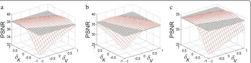
Figure 5Dependences of PSNR onδVandδkfor the test image #3.For different noise cases:k= 0.2;σ2
si= 10(a),k= 0.2;σ2si= 50(b), and
overestimation of both parameters of the mixed noise, oversmoothing is observed. It mainly appears itself in smearing low contrast texture (bushes) in the central part of the picture in Figure 3d. The reduction of the metric MSSIM is observed as well. For the case consi-dered in Figure 3, reduction is equal to 0.004.
Besides, Figure 4 represents images for another case. The simple structure image #3 (its noise-free color ver-sion is presented in Figure 4a) is corrupted by rather in-tensive signal-dependent noise with σ2
si = 30 and k= 1.0
(Figure 4b, red component). Noise is well visible, espe-cially in image homogeneous regions. Figure 4c presents the denoised image under assumption that mixed noise parameters are estimated absolutely accurately. Mean-while, Figure 4d represents the output image obtained in the case of underestimation of mixed noise parameters. As it is seen, underestimation leads to residual noise that appears itself clearly in image homogeneous regions. Again, reduction of PSNR and PSNR-HVS-M is close to 0.5 dB while decrease of MSSIM is close to 0.005.
Thus, both underestimation and overestimation of the mixed noise parameters are undesirable. Underestima-tion is crucial for simple structure images and overesti-mation is undesired for complex structure images.
We have checked other test images and other noise par-ameter sets. Analysis carried out for all images in TID2008 has shown that reduction of PSNR and PSNR-HVS-M by about 0.5 dB approximately corresponds to MSSIM reduc-tion by 0.005. Note that all three dependences are non-linear and there is no strict relationship between them. The only observation is that if PSNR-HVS-M decreases, MSSIM usually diminishes as well and vice versa.
Thus, our approach to analysis consists in the following. The first task is to determine 2D areas ofδVandδkwhere reduction is smaller than 0.5 dB according to the metrics PSNR and PSNR-HVS-M or smaller than 0.005 according to MSSIM for each considered image and each set of mixed noise parameters. It is assumed that if the mixed noise pa-rameters’ estimates are within these areas, the estimation errors do not essentially influence the filtering accuracy.
Note that in addition to three aforementioned sets of mixed noise parameters for the model (1), we consider below one set (combination) of σ2
si and kfor the model
(2) to simulate the real-life situation for which the multi-plicative noise is dominant. Then, at the second stage, the obtained areas have to be aggregated by AND rule to provide final requirements to estimation accuracy under assumption that neither noise statistics nor image pro-perties are available in advance.
4. Analysis of results
The obtained dependences of output PSNR on δVand δk are presented as 2D surfaces (see Figure 5) of red color. Black color horizontal surface corresponds to the levels PSNR(δV= 0, δk= 0)−0.5, dB and PSNR-HVS-M(δV= 0,
δk= 0)−0.5, dB, respectively. Thus, it is easy to see for which area ofδVandδkfiltering efficiency is acceptable for each particular case (red color surface is over black one).
Three combinations of k and σ2
si are considered,
namely,k= 0.2,σ2si= 10;k= 0.2,σ2si = 50; andk= 1,σ2si= 30. For each combination, Table 1 presents the following data: MSEinp to discriminate the cases of dominant signal-dependent or signal-independent noise; PSNR (δV=−1, δk=−1), i.e., for original noisy image; PSNR (δV= 0, δk= 0), i.e., for the image filtered with the re-commended parameter under condition of absolutely ac-curate estimation of σ2
si and k; max PSNR, i.e., maximal attained value and the values δVmax, δkmax for which maxPSNRhas been provided.
Table 2 Simulation data for the test image #3, noise model (1), PSNR-HVS-M metric
k σ2
si MSEinp PSNR-HVS-M
(δV=−1,
δk=−1)
PSNR-HVS-M (δV=−0,
δk=−0)
maxPSNR− HVS−M
δVmaxvis δkmaxvis
0.2 10 32.66 36.32 40.29 40.30 0.2 −0.1
0.2 50 72.62 32.45 37.45 37.47 0.2 −0.5
1.0 30 144.01 29.22 34.67 34.68 0.7 −0.2
Figure 6Dependences of PSNR-HVS-M onδVandδkfor the test image #3.For different noise cases:k= 0.2;σ2si= 10(a),k= 0.2;σ2si= 50(b),
As it is seen, for two cases (k= 0.2,σ2si= 10 andk= 1,
σ2
si = 30), the SD noise component is dominant (MSEinp>2
σ2
si). For the casek= 0.2, σ2si = 50, the SI noise
compo-nent is dominant. The first observation is that if noise is more intensive (compare the case k= 1, σ2
si = 30 to the
case k= 0.2, σ2si = 10), the DCT-based filtering is more efficient (PSNR(δV= 0,δk= 0) differs more from the cor-responding PSNR(δV=−1,δk=−1)). In particular, PSNR (δV= 0, δk= 0) is larger by about 8 dB than PSNR (δV=−1,δk=−1) for the casek= 1,σ2
si= 30.
If the SD noise component is dominant (see the plots in Figure 5a, c), it does not matter too much how accu-rate the estimatesσ^2
siare. It is considerably more
impor-tant how accurate is the estimate of the SD noise parameter k. If ^σ2
si is quite accurate (let us say, |δV|≤
0.5), then |δk| should be smaller than about 0.4. Thus, if the SD noise component is dominant, then the requirement to accuracy ofkis stricter than the requirement to accuracy ofσ^2
si. This appears itself in the fact that a red surface‘strip’
that is ‘over’ the corresponding threshold (black color surface) is oriented more parallel to the axisδV.
Another situation is observed if SI noise component is dominant (see the plot in Figure 5b). Then accuracy of estimating the parameterkis less important, but the re-quirement to estimation of σ2
si is stricter. In fact, for the
considered case, it is desirable to provide |δV| less than 0.3…0.4. The red surface‘strip’is oriented more parallel to the axisδk. Thus, initial conclusion is quite trivial - it is necessary to more accurately estimate the parameter for the noise component which is dominant.
If one parameter is overestimated, then it is desirable to have another parameter underestimated (⌢k <k) to provide rather efficient filtering (see the values δVmax and δkmax in Table 1). It is better, if ⌢σsi2 >σ2si;δV >0 . The worst case is if both parameters, σ2
si and k, are
underestimated. Then, undersmoothing is observed (look at data for δV→−1, δk→−1) and filtering effi-ciency is far from optimal (attainable). One more inter-esting observation that follows from analysis of data in Table 1 is that maxPSNRis only slightly (by 0.01…0.05 dB) larger than PSNR(δV= 0,δk= 0). This shows that the prac-tical recommendation (5) works well enough.
Consider now the dependences for the metric PSNR-HVS-M presented in Figure 6. The corresponding data are collected in Table 2. For each combination, Table 2 presents the values of PSNR-HVS-M(δV=−1,δk=−1)for original noisy images; PSNR-HVS-M(δV= 0, δk= 0), i.e., for the images filtered with the recommended parameter under condition of absolutely accurate estimation of σ2
si
andk; maxPSNR−HVS−M, i.e., maximal reachable value and the values δVmaxvis, δkmaxvis for which maxPSNR−HVS−M has been attained.
From the very beginning, let us stress that the values PSNR-HVS-M(δV=−1,δk=−1) are larger than the cor-responding PSNR(δV=−1, δk=−1). This is due to the masking effects [39]. As it is according to the metric PSNR, PSNR-HVS-M increases for the recommended set-ting of the DCT filter parameterβ(compare PSNR-HVS-M (δV= 0, δk= 0) to PSNR-HVS-M(δV=−1, δk=−1)). Visual quality improvement due to filtering is essential - from
Table 3 Simulation data for the test image #13, noise model (1), PSNR metric
k σ2
si MSEinp PSNR (δV=
−1,δk=−1)
PSNR (δV=
−0,δk=−0)
maxPSNR δVmax δkmax
0.2 10 32.0 33.08 33.91 33.96 −0.6 0
0.2 50 71.93 29.56 30.99 31.09 −0.3 0
1.0 30 140.24 26.66 28.64 28.77 −0.6 −0.1
Table 4 Simulation data for the test image #13, noise model (1), PSNR-HVS-M metric
k σ2
si MSEinp PSNR-HVS-M
(δV=−1,
δk=−1)
PSNR-HVS-M (δV=−0,
δk=−0)
maxPSNR− HVS−M
δVmaxvis δkmaxvis
0.2 10 32.0 40.08 40.36 40.45 −0.1 −0.4
0.2 50 71.93 34.90 35.42 35.56 −0.4 0
1.0 30 140.24 31.30 32.01 32.24 −0.7 −0.2
c
b
a
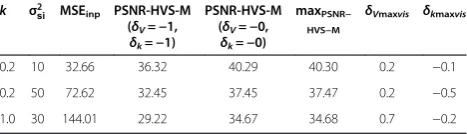
Figure 7Dependences of MSSIM onδVandδkfor the R component of the test image #3.For different noise cases:k= 0.2;σ2si= 10(a),k=
0.2;σ2
about 4 dB for non-intensive noise (k= 0.2; σ2si = 10), it reaches 5.5 dB for the case k= 1, σ2
si = 30. Note that
PSNR-HVS-M(δV= 0,δk= 0) fork= 0.2; σ2si = 10 exceeds 40 dB, i.e., residual distortions in the filtered image are almost invisible [35].
The observed values maxPSNR−HVS−M practically do not differ from the corresponding PSNR-HVS-M(δV= 0,
δk= 0). Interestingly, all δVmaxvis are larger than 0 while
all δkmaxvisare smaller than 0. This means that it is less
risky to overestimate SI noise variance and underesti-mate the parameterkthan to fall into other possible sit-uations. Meanwhile, all δVmaxvis (Table 2) are smaller
than the corresponding δVmax(see Table 1). This shows that for providing higher visual quality, it is undesirable to have considerable overestimation of mixed noise pa-rameters. In some sense, it is equivalent to the recom-mendation to have β slightly smaller than 2.6 in threshold setting (5) to guarantee good visual quality of filtered image [38].
Figure 7 shows dependences of the metric MSSIM on
δV and δk for the test image #3. The conclusions that can be drawn from their analysis are similar to those presented above. Overestimation of mixed noise parame-ters is less risky than underestimation. It is more impor-tant to correctly estimate the parameter of mixed noise
that corresponds to the dominant component of the noise.
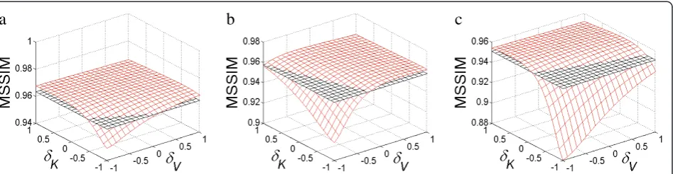
Consider now the results for the test image #13 (Figures 1 or 3a). Again, we present data only for R com-ponent processed but the dependences for other color components are very similar. The dependences obtained for PSNR and PSNR-HVS-M are represented in Figures 8 and 9, respectively. Particular data are collected in Tables 3 and 4. Note that the casesk= 0.2,σ2si = 10 and k= 1;σ2
si= 30, as earlier, correspond to the dominant SD
noise component while the SI noise component is prevailing if k= 0.2; σ2si = 50.
At the first glance, the dependences in Figures 8 and 9 are quite similar to the corresponding dependences in Figures 5 and 6. However, there are several distinctive differences. One of them is that filtering of the test image #13 is considerably less efficient than of the test image #3. Only for the most intensive noise (k= 1; σ2
si =
30), the difference between PSNR(δV= 0, δk= 0) and PSNR for the original image (PSNR(δV=−1, δk=−1)) reaches 2 dB. This difference is only 0.83 dB for the case k= 0.2;σ2
si = 10. The value maxPSNRis 0.05…0.13 dB larger than the corresponding PSNR(δV= 0,δk= 0), and this takes place ifδVmax< 0, i.e., if SI noise variance is underestimated and the parameterkis estimated properly (without error).
c
b
a
Figure 8Dependences of PSNR onδVandδkfor the R component of the test image #13.For different noise cases:k= 0.2;σ2
si= 10(a),k=
0.2;σ2
si= 50(b), andk= 1;σ2si= 30(c).
c
b
a
Figure 9Dependences of PSNR-HVS-M onδVandδkfor the R component of the test image #13.For different noise cases:k= 0.2;σ2si= 10 (a),k= 0.2;σ2
Overestimation of both parameters is severely undesir-able since this leads to reduction of filtering efficiency and image oversmoothing (analyze data forδV→1,δk→ 1 where the dependences PSNR(δV, δk) rapidly decrease ifδVandδkincrease).
Analysis of plots in Figure 9 and data in Table 4 leads to the same conclusions. Note that in the case k= 0.2;
σ2
si= 10, PSNR-HVS-M increase due to filtering is only
0.28 dB, i.e., it is practically invisible. Only for k= 1;
σ2
si = 30 the value PSNR-HVS-M(δV= 0, δk= 0) is by
0.71 dB larger than for the original image, i.e., there is a small noticeable improvement of visual quality. This means that if filtering is applied to improve visual quality of highly textural images based on mixed noise parameters estimated in a blind manner, then these es-timates should not be essentially larger than true values of these parameters (i.e., in fact, it is desirable to haveδV≤0,δk≤0).
c
b
a
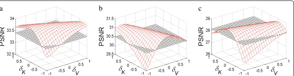
Figure 10Dependences of MSSIM onδVandδkfor the R component of the test image #13.For different noise cases:k= 0.2;σ2si= 10(a),
k= 0.2;σ2
si= 50(b), andk= 1;σ2si= 30(c).
-1 -0.8 -0.6 -0.4 -0.2 0 0.2 0.4 0.6 0.8 1 -1
-0.8 -0.6 -0.4 -0.2 0 0.2 0.4 0.6 0.8 1
δV δV
δV δV
δ K δ K
δ K
δ K
-1 -0.8 -0.6 -0.4 -0.2 0 0.2 0.4 0.6 0.8 1 -1
-0.8 -0.6 -0.4 -0.2 0 0.2 0.4 0.6 0.8 1
b
a
-1 -0.8 -0.6 -0.4 -0.2 0 0.2 0.4 0.6 0.8 1 -1
-0.8 -0.6 -0.4 -0.2 0 0.2 0.4 0.6 0.8 1
-1 -0.8 -0.6 -0.4 -0.2 0 0.2 0.4 0.6 0.8 1 -1
-0.8 -0.6 -0.4 -0.2 0 0.2 0.4 0.6 0.8 1
d
c
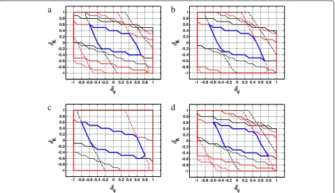
Figure 11Areas of acceptableδVandδkfor different noise cases with marked boundaries for appropriate estimation accuracy. (a)For
PSNR;(b)for PSNR-HVS-M and(c)for MSSIM metrics for red color component and(d)for PSNR for green color component. Notations used: black color for image #3, red color for image #13, solid line for the casek= 1;σ2
si= 30; dashed line for the casek= 0.2;σ2si= 10; dashed-dotted line for
Figure 10 presents the obtained results for the metric MSSIM. Their analysis also shows that overestimation of mixed noise parameters is severely undesirable for this (highly textural) test image. Parameter that relates to a dominant component of the mixed noise has to be esti-mated more accurately.
Let us now aggregate the obtained results for three noise parameter combinations and two test images of sufficiently different complexity. For this purpose, we have marked the ‘allowed’2D areas of mixed noise par-ameter estimates to be acceptable (see Figure 11 and de-scription of notations used) and determined a joint acceptable area (where all areas overlap). This area is in-dicated by solid (blue) line and is located in the central part (horizontal axis corresponds to δV and vertical to
δk). Although all particular areas are of rather large size, their intersection is, certainly, smaller. However, it is still quite large. In the worst case, |δk| = 0.2 and |δV| = 0.3 (see Figure 11a). The conclusions that can be drawn from analysis of the area according to the metric PSNR-HVS-M (Figure 11b) are practically the same. The inter-section area obtained for the metric MSSIM (Figure 11c) almost coincides with that for the metric PSNR.
To show that the results obtained for other color com-ponents are similar to the results obtained for the red component, Figure 11d presents intersection areas for the green component according to the metric PSNR. Comparison of the obtained acceptable areas to the cor-responding areas presented in Figure 11a shows that there is no essential difference.
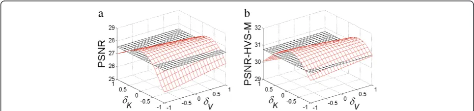
Let us consider now the data for the model (2). Only one case has been simulated: k= 0.01, σ2si = 20. The de-pendences of PSNR and PSNR-HVSM onδVand δkfor the R component of the test image #3 are presented in Figure 12. The data are collected in Tables 5 and 6.
As it is seen, the multiplicative noise is dominant. Be-cause of this, the parameter k has to be estimated with higher accuracy than the parameter σ2
si. PSNR and
PSNR-HVS-M improvement due to filtering is quite large, about 8 dB for PSNR and about 5 dB for
PSNR-HVS-M. Similarly, Figure 13 presents dependences of PSNR and PSNR-HVS-M onδVandδkfor the R compo-nent of the test image #13.
The data are given in Tables 5 and 6, respectively. In this case, PSNR and PSNR-HVS-M improvement for ac-curately estimated kand σ2si (see data for δV= 0, δk= 0) is considerably smaller than for the test image #3. The requirement to accuracy of the parameterkestimation is stricter than to estimation accuracy of the parameter σ2
si
although the estimation errors with |δk|≤0.2 are still acceptable. Overestimation of the parameter k is es-pecially undesirable.
A shortcoming of the analysis carried out above is that only two test images (although with essentially different properties) and only four (totally) sets of mixed noise parameters (although quite different) have been consi-dered. Thus, let us also study two extreme cases. Ac-cording to the previous analysis, the strictest restrictions are observed for the following cases: (a) a complex struc-ture image corrupted by non-intensive noise with obvi-ous dominance of one component, for example, additive; (b) a simple structure image corrupted by intensive noise with one prevailing component, for example, signal dependent of the model (2).
For the case a, we have used the test image #1 from the database TID2008 (Figure 1). The model (1) noise has been simulated with k= 0.01 and σ2si = 25. These settings relate to, e.g., the practical case of noisy (junk) component images acquired by old generation hyper-spectral sensors [8]. For the case b, the test image #23 from TID2008 (Figure 1) that is one of the simplest Figure 12Dependences of PSNR (a) and PSNR-HVS-M (b) onδVandδkfor the test image #3.With noise simulated according model (2) for
k= 0.01 andσ2 si= 20.
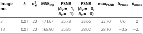
Table 5 Simulation data for the test image #3 and 13, noise model (2), PSNR metric
Image
no. k σ
2
si MSEinp PSNR (δV=−1,
δk=−1) PSNR (δV=−0, δk=−0)
maxPSNR δVmax δkmax
3 0.01 20 171.67 25.78 33.66 33.70 0.6 0
has been exploited. The model (2) noise has been gen-erated withk= 0.1 andσ2
si = 10. Such noise can be
ob-served in images formed by multi-look synthetic aperture radars.
The obtained dependences of PSNR, PSNR-HVS-M, and MSSIM onδVand δkfor the case a are presented in Figure 14. Obviously, σ2si has to be estimated with high accuracy and its overestimation is strongly undesirable. Quality improvement due to filtering is small even for the best settings.
The dependences for the case b are shown in Figure 15. It is seen that the parameterk has to be estimated cor-rectly. Its underestimation can lead to considerable undersmoothing and is undesirable. In both extreme cases, it is still enough to estimate the dominant noise parameter with relative error not exceeding 0.2.
Finally, we have obtained intersection areas for two metrics (PSNR and PSNR-HVS-M) for all images (three components for each image) and all considered sets of signal-dependent noise models. These areas are shown in Figure 16. The first observation is that these accep-table areas are only slightly smaller than those ones pre-sented earlier in Figure 11. Conclusions that follow from the analysis of these areas are the following. First, abso-lute values of both errors δV and δk should not, in ge-neral, be larger than 0.2. Second, as exceptional situation, it is possible that absolute values of one of these errors can be slightly larger than 0.2 (but in this case, another error should have the opposite sign). This property appears itself in non-circular (quasi-elliptical shape of acceptable areas). Third, the acceptable area for the metric PSNR-HVS-M is slightly shifted with respect
to the acceptable area for the metric PSNR toward smaller values of both errors. In fact, this means that overestimation of mixed noise parameters is more risky for providing high visual quality of filtered images com-pared to the case of conventional analysis of denoising efficiency in terms of output MSE or PSNR.
Clearly, the way we followed in our analysis is not the only one possible. It is also possible to study tolerance of filtering techniques to ambiguity or inaccuracy of available a priori information in other ways. One of them can be based on simulating some estimates of noise parameters and using them instead of true values in denoising with statistical assessment of filtering efficiency. Following this way, we have assumed unbiased estimation of both parameters for the noise model (1) and estimates modeled as k^¼kþΔk; ^σ2
si¼^σ2siþΔσ^si2; where Δk and Δσ^2si
are mutually independent zero mean random variables supposed to be Gaussian with standard deviations δk and δv, respectively. Then, varyingδk, δv, it is possible to simulate erroneous estimation for a set of realiza-tions, to determine what are filtering criteria values (PSNR, PSNR-HVS-M, MSSIM) for each realization and to statistically process them with obtaining mean and standard deviation for each considered metric as well as confidence intervals.
Note that erroneous estimation of noise parameters leads to degradation of all metrics (reduction of their mean values compared to the corresponding optimal ones). Because of this, we have determined confidence interval width as MCW = |MO−MM| + 3MS, where MO determines optimal value of a visual quality metric for errorless noise parameters estimates; MM is mean
Table 6 Simulation data for the test image #3 and 13, noise model (2), PSNR-HVS-M metric
Image No k σ2
si MSEinp PSNR-HVS-M (δV=−1,δk=−1) PSNR-HVS-M (δV=−0,δk=−0) maxPSNR−HVS−M δVmaxvis δkmaxvis
3 0.01 20 171.67 28.46 33.48 33.49 0.6 −0.1
13 0.01 20 168.90 30.32 31.24 31.39 −0.8 −0.2
b
a
Figure 13Dependences of PSNR (a) and PSNR-HVS-M (b) onδVandδkfor the test image #13.With noise simulated according model (2) fork= 0.01 andσ2
value of a visual quality metric; MS is standard deviation of a visual quality metric.
Simulation results for the test images #3 and #13 for two sets of parameters for model (1) are presented in Table 7. Recall that we need MCW less than 0.5 dB for the metrics PSNR and PSNR-HVS-M and less than 0.005 for the metric MSSIM. Conditions for which these requirements are satisfied depend upon a test image and noise parameters. The larger values of δk, δv result in larger degradations of all metrics. However, the afore-mentioned requirements are usually satisfied if both
δk, δv are smaller than 0.15. If these standard devia-tions are both equal to 0.25, requirements can be not satisfied. Thus, we come approximately to the same conclusions as in our previous analysis.
5. Conclusions and future work
The question of influence of mixed noise parameters es-timation accuracy on filtering efficiency in image en-hancement applications is studied. It is demonstrated that the parameter that corresponds to a dominant noise type has to be estimated with a higher accuracy. This ac-curacy is characterized by a relative error that should be less than 20% for the dominant noise type and less than 30% for another type of noise. Then, decrease of filtering
efficiency characterized by PSNR or PSNR-HVS-M drop compared to the optimum does not exceed 0.5 dB (MSSIM drop does not exceed 0.005), and thus, it is practically not noticeable (crucial). Note that these re-quirements practically coincide with rere-quirements to ac-curacy of pure additive or pure multiplicative noise variance estimation [17] - an estimate has to differ from a true value by less than 20%. It is also important to stress that even the most advanced modern methods of blind estimation of mixed noise parameters do not al-ways provide the required accuracy of parameters’ estimation [44].
It is also shown that for highly textural images it is better to have underestimation of the mixed noise pa-rameters than overestimation. Unfortunately, it happens in practice that mixed noise parameters are usually over-estimated for complex structure images [22]. This moti-vates a design of more accurate methods for blind estimation including analysis of dependences between the estimates of components of the mixed noise.
Besides, in the future, we plan to concentrate on con-sidering spatially correlated noise which is rather typical in practice. Other filters based on using estimated pa-rameters of mixed noise can be studied as well since re-strictions for them can differ from rere-strictions obtained for the DCT-based denoising.
c
b
a
Figure 14Dependences of PSNR (a), PSNR-HVS-M (b), and MSSIM (c) onδVandδkfor the test image #1.With noise simulated according model (1) fork= 0.01 andσ2
si= 25.
c
b
a
Figure 15Dependences of PSNR (a), PSNR-HVS-M (b), and MSSIM (c) onδVandδkfor the test image #23.With noise simulated according
-0.5 -0.4 -0.3 -0.2 -0.1 0 0.1 0.2 0.3 0.4 0.5 -0.5
-0.4 -0.3 -0.2 -0.1 0 0.1 0.2 0.3 0.4 0.5
-0.5 -0.4 -0.3 -0.2 -0.1 0 0.1 0.2 0.3 0.4 0.5 -0.5
-0.4 -0.3 -0.2 -0.1 0 0.1 0.2 0.3 0.4 0.5
b
a
δV δV
δ K δ K
Figure 16Areas of acceptableδVandδkfor two metrics. (a)PSNR and(b)PSNR-HVS-M for all TID2008 database images (three components
for each image) and all considered sets of signal-dependent noise models.
Table 7 Simulation data for the test image #3 and 13, noise model (1), all considered metrics
δk,δν PSNR PSNR-HVS-M MSSIM
MO MM MS MCW MO MM MS MCW MO MM MS MCW
Image 03
Casek= 0.2;σ2 si= 50
0.05 36.58 36.57 0.013 0.046 37.40 37.40 0.006 0.017 0.9841 0.9841 0.0001 0.0002
0.10 36.55 0.045 0.160 37.38 0.030 0.103 0.9840 0.0002 0.0007
0.15 36.52 0.103 0.364 37.37 0.059 0.207 0.9839 0.0005 0.0016
0.20 36.49 0.158 0.557 37.34 0.091 0.328 0.9838 0.0007 0.0025
0.25 36.41 0.244 0.900 37.29 0.142 0.534 0.9834 0.0011 0.0041
Casek= 1.0;σ2 si= 30
0.05 34.53 34.52 0.020 0.065 34.67 34.67 0.004 0.018 0.9756 0.9764 0.0002 0.0005
0.10 34.51 0.051 0.173 34.66 0.026 0.095 0.9764 0.0004 0.0012
0.15 34.44 0.132 0.480 34.63 0.071 0.260 0.9760 0.0009 0.0031
0.20 34.37 0.336 1.162 34.58 0.189 0.662 0.9756 0.0023 0.0077
0.25 34.35 0.347 1.218 34.56 0.198 0.710 0.9755 0.0023 0.0079
Image 13
Casek= 0.2;σ2 si= 50
0.05 31.00 31.00 0.034 0.102 35.42 35.42 0.046 0.138 0.9828 0.9828 0.0003 0.0008
0.10 30.98 0.066 0.215 35.40 0.087 0.277 0.9827 0.0005 0.0016
0.15 30.96 0.100 0.343 35.37 0.126 0.426 0.9825 0.0008 0.0025
0.20 30.97 0.151 0.479 35.40 0.194 0.598 0.9827 0.0012 0.0036
0.25 30.93 0.164 0.555 35.36 0.217 0.709 0.9825 0.0013 0.0043
Casek= 1.0;σ2 si= 30
0.05 28.64 28.64 0.041 0.127 32.01 32.01 0.054 0.164 0.9713 0.9713 0.0005 0.0017
0.10 28.64 0.080 0.246 32.01 0.101 0.308 0.9712 0.0010 0.0031
0.15 28.61 0.109 0.356 31.98 0.137 0.443 0.9710 0.0014 0.0045
0.20 28.62 0.143 0.450 32.00 0.185 0.563 0.9713 0.0019 0.0059
Competing interests
The authors declare that they have no competing interests.
Author details
1National Aerospace University, Kharkov 61070, Ukraine.2Tampere University
of Technology, Tampere FI-33101, Finland.
Received: 29 March 2013 Accepted: 23 December 2013 Published: 14 January 2014
References
1. WK Pratt,Digital Image Processing, 4th edn. (Wiley-Interscience, New York, 2007). p. 807
2. M Elad, Sparse and Redundant Representations, inFrom Theory to Applications in Signal and Image Processing, ed. by M Elad. vol. 20 (Springer Science, Business Media, LLC, Philadelphia, PA, 2010), p. 376 3. OK Al-Shaykh, RM Mersereau, Lossy compression of noisy images. IEEE Trans.
on Image Process.7(12), 1641–1652 (1998). doi:10.1109/83.730376 4. A Bovik,Handbook on Image and Video Processing(Waltham, MA, Academic
Press, 2000), p. 1384
5. DL Donohо, De-noising by soft thresholding. IEEE Trans. on Information TheoryIT-41(3), 613–627 (1995)
6. S Mallat,A Wavelet Tour of Signal Processing(Academic, San Diego, CA, 1998), p. 620
7. L Sendur, IW Selesnick, Bivariate shrinkage with local variance estimation. IEEE Sig. Process. Letters9(12), 438–441 (2002)
8. V Lukin, S Abramov, N Ponomarenko, M Uss, M Zriakhov, B Vozel, K Chehdi, J Astola, Methods and automatic procedures for processing images based on blind evaluation of noise type and characteristics. SPIE J. Adv. Remote Sens (2011). doi: 10.1117/1.3539768
9. A Foi,Pointwise Shape-Adaptive DCT Image Filtering and Signal-Dependent Noise Estimation, Thesis for the degree of Doctor of Technology
(Tampere University of Technology, Tampere, 2007)
10. C Oliver, S Quegan,Understanding Synthetic Aperture Radar Images
(Raleigh, NC, SciTech Publishing, 2004), p. 479
11. N Ponomarenko, V Lukin, K Egiazarian, L Lepisto, Color image lossy compression based on blind evaluation and prediction of noise characteristics, inProceedings of the SPIE 7870 of Image Processing: Algorithms and Systems VII(San Francisco, 23 Jan 2011)
12. C Liu, R Szeliski, SB Kang, CL Zitnick, WT Freeman, Automatic estimation and removal of noise from a single image. IEEE Trans. Pattern Anal. Mach. Intell. 30(2), 299–314 (2008)
13. SH Lim, Characterization of Noise in Digital Photographs for Image Processing, inProceedings of the SPIE 6069 of Digital Photography II
(San Jose, 15 Jan 2006)
14. PJ Curran, JL Dungan, Estimation of signal-to-noise: a new procedure applied to AVIRIS data. IEEE Trans. Geosci. Remote Sens.27, 620–628 (1989) 15. M Uss, B Vozel, V Lukin, K Chehdi, Local signal-dependent noise variance
estimation from hyperspectral textural images. IEEE J. Select. Topics Signal Process5, 469–486 (2011)
16. B Aiazzi, L Alparone, A Barducci, S Baronti, P Marcoinni, I Pippi, M Selva, Noise modelling and estimation of hyperspectral data from airborne imaging spectrometers. Ann. Geophys.49, 19 (2006)
17. B Vozel, S Abramov, K Chehdi, V Lukin, N Ponomarenko, M Uss, J Astola, Multivariate Image Processing, inBlind Methods for Noise Evaluation in Multi-Component Images, ed. by C Collet, J Chanussot, K Chehdi (Toulouse, Wiley&Iste, 2010), pp. 263–302
18. S Abramov, V Lukin, N Ponomarenko, K Egiazarian, O Pogrebnyak, Influence of multiplicative noise variance evaluation accuracy on MM-band SLAR image filtering efficiency, inProceedings of the MSMW 2004. vol 1, (Kharkov, 21–26 Jun 2004), pp. 250–252
19. JP Kerekes, JE Baum, Hyperspectral imaging system modeling. Lincoln Laboratory J.14(1), 117–130 (2003)
20. A Barducci, D Guzzi, P Marcoionni, I Pippi, CHRIS-Proba performance evaluation: signal-to-noise ratio, instrument efficiency and data quality from acquisitions over San Rossore (Italy) test site, inProceedings of the 3rd ESA CHRIS/Proba Workshop, 21–23 Mar 2005
21. S Abramov, V Zabrodina, V Lukin, B Vozel, K Chehdi, J Astola, Improved method for blind estimation of the variance of mixed noise using weighted LMS line fitting algorithm, inProceedings of the ISCAS(Paris, 30 May–2 Jun 2010), pp. 2642–2645
22. S Abramov, V Zabrodina, V Lukin, B Vozel, K Chehdi, J Astola, Methods for Blind Estimation of the Variance of Mixed Noise and Their Performance Analysis, inNumerical Analysis–Theory and Applications, ed. by J Awrejcewicz (Richardson, TX, InTech, 2011), pp. 49–70. doi: 10.5772/1829 23. D Fevralev, V Lukin, N Ponomarenko, S Abramov, K Egiazarian, J Astola,
Efficiency analysis of color image filtering. EURASIP J. Adv. Signal Process. 2011, 41 (2011). doi:10.1186/1687-6180-2011-41
24. R Oktem, K Egiazarian, Transform domain algorithm for reducing the effect of film-grain noise in image compression. Electronic Letters35(21), 1830–1831 (1999) 25. G Ramponi, R D’Alvise, Automatic Estimation of the Noise Variance in SAR Images
for Use in Speckle Filtering, inProceedings of the IEEE-EURASIP Workshop on Non-linear Signal and Image Processing(Antalya, 20–23 Jun 1999), pp. 835–838 26. J Astola, P Kuosmanen,Fundamentals of nonlinear digital filtering
(CRC Press LLC, Boca Raton, 1997). 276
27. VI Ponomaryov, Real time 2D-3D filtering using order statistics based algorithms. J. of Real-Time Image Process.1, 173–194 (2007)
28. V Lukin, N Ponomarenko, S Abramov, B Vozel, K Chehdi, Improved noise parameter estimation and filtering of MM-band SLAR images, inProceedings of the MSMW 2007. vol 1, (Kharkov, 25–30 Jun 2007), pp. 439–441 29. KN Plataniotis, AN Venetsanopoulos,Color Image Processing and Applications
(Springer, New York, 2000). 355
30. J Astola, P Haavisto, Y Neuvo, Vector median filter. Proc. IEEE4, 678–689 (1990) 31. R Touzi, A review of speckle filtering in the context of estimation theory.
IEEE Trans. on Geosci. and Remote Sens.40(11), 2392–2404 (2002) 32. A Foi, Clipped noisy images: heteroskedastic modeling and practical
denoising. Signal Process.89(12), 2609–2629 (2009)
33. F Murtagh, JL Starck, A Bijaoui, Image restoration with noise suppression using a multiresolution support. Astron. Astrophys. Suppl. Ser.112, 179–189 (1995) 34. V Lukin, N Ponomarenko, S Abramov, B Vozel, K Chehdi, J Astola, Filtering of
radar images based on blind evaluation of noise characteristics, in
Proceedings of the Image and Signal Processing for Remote Sensing XIV. vol 7109 (Cardiff, 15–18 Sep 2008)
35. R Oktem, K Egiazarian, VV Lukin, NN Ponomarenko, OV Tsymbal, Locally adaptive DCT filtering for signal-dependent noise removal. EURASIP J. Adv. Signal Process (2007). doi:10.1155/2007/42472
36. D Fevralev, S Krivenko, V Lukin, A Zelensky, K Egiazarian, Speeding-up DCT based Filtering of Images, inCD ROM Proceedings of the Modern Problems of Radioengineering, Telecommunications and Computer Science (TCSET) (Lviv-Slavsko, 23–27 Feb 2010)
37. K Dabov, A Foi, V Katkovnik, K Egiazarian, Image denoising by sparse 3-D transform-domain collaborative filtering. IEEE Trans. Image Process.16(8), 2080–2095 (2007)
38. V Lukin, N Ponomarenko, K Egiazarian, HVS-Metric-Based Performance Analysis Of Image Denoising Algorithms, inProceedings of the EUVIP(Paris, 4–6 Jul 2011) 39. N Ponomarenko, F Silvestri, K Egiazarian, M Carli, J Astola, V Lukin, On
between-coefficient contrast masking of DCT basis functions, inCD-ROM Proceedings of the VPQM(Scottsdale, 25–26 Jan 2007)
40. N Ponomarenko,PSNR-HVS-M download page, 2009. http://www. ponomarenko.info/psnrhvsm.htm. Accessed 28 Mar 2013 41. N Ponomarenko, V Lukin, A Zelensky, K Egiazarian, M Carli, F Battisti,
TID2008 - a database for evaluation of full-reference visual quality assessment metrics. Advances of Modern Radioelectronics10, 30–45 (2009)
42. V Lukin, M Zriakhov, S Krivenko, N Ponomarenko, Z Miao, Lossy compression of images without visible distortions and its applications, in
Proceedings of the ICSP 2010(Beijing, 24–28 Oct 2010), pp. 694–697 43. Z Wang, EP Simoncelli, AC Bovik, Multi-scale Structural Similarity for Visual
Quality Assessment, inProceedings of the 37th IEEE Asilomar Conference on Signals, Systems and Computers. vol 2 (Monterey, 9–12 Nov 2003), pp. 1398–1402 44. ML Uss, B Vozel, V Lukin, K Chehdi, Image Informative Maps for
Component-wise Estimating Parameters of Signal-Dependent Noise. J. Electron. Imag22(1) (2013). doi:10.1117/1.JEI.22.1.013019
doi:10.1186/1687-5281-2014-3
Cite this article as:Abramovaet al.:On required accuracy of mixed noise parameter estimation for image enhancement via denoising.