http://www.sciencepublishinggroup.com/j/ijass doi: 10.11648/j.ijass.20190704.12
ISSN: 2376-7014 (Print); ISSN: 2376-7022 (Online)
Comparison of Global Vertical Total Electron Content from
Various Global Data Centers
Shambel Gizachew
1, Belay Sitotaw
1, Gizaw Mengistu Tsidu
21Physics Department, Dire Dawa University, Dire Dawa, Ethiopia 2
Physics Department, Addis Ababa University, Addis Ababa, Ethiopia
Email address:
To cite this article:
Shambel Gizachew, Belay Sitotaw, Gizaw Mengistu Tsidu. Comparison of Global Vertical Total Electron Content from Various Global Data Centers. International Journal of Astrophysics and Space Science. Vol. 7, No. 4, 2019, pp. 50-57. doi: 10.11648/j.ijass.20190704.12
Received: March 26, 2019; Accepted: April 26, 2019; Published: October 23, 2019
Abstract:
In this study, the inter-comparison of various global vertical total electron contents are derived from Global Positioning System (GPS) networks worldwide. Based on observation data obtained from global network of dual frequency, the ionospheric variability on one full year, 2008 is studied through the vertical electron conten distribution GPS. The comparisons are aimed at comparability of the different vertical total electron content data sets in terms of absolute magnitude, capturing diurnal, seasonal variability globally. Total electron content (TEC) values were compared by computing the TEC differences among different stations. Most of the data sets exhibit expected diurnal variability with some differences on the absolute magnitude of vertical total electron content moreover, seasonally, the variability is also comparable. In this observation, highest vertical electron contents are observed on the Jet prolusion laboratory. It is followed by International global service, vertical total electron content and the least is observed on the Polytechnical University data sets.Keywords:
Vertical Electron Content, Diurnal, Seasonal Variation, GPS1. Introduction
There are regions of the atmosphere which are defined by the variation of temperature. They are defined by the temperature structure, density, composition, and degree of ionization. Throughout the atmosphere temperature varies with altitude, and so the different regions are defined by temperature. Various natural or artificial phenomena which may result from the different forms of energy and physical mechanisms present in the atmosphere occur in and/or propagate through the atmosphere [1].
Global Positioning System (GPS) satellites in high altitude orbits (~20,200 km) are capable of providing details on the structure of the entire ionosphere, even the plasmasphere. Nowadays, GPS has become the most widely used tool for investigations of ionospheric irregularities due to the lowcost, all-weather, near real time, and high-temporal resolution (30s) technique. Mapping TEC with GPS has been reported in the literatures and their application to space climate was successfully carried out by many countries’ scientists [2].
A number of investigations have been used one of GPS
data sets in the past. While the basis of selection of one data set over the other for a given study has never been formally presented, there is a need to know their relative accuracy and advantages over each other for the sake of comparing results of past and future studies. This study is conducted to fill this information gap and assess the level of agreements between different data sets so that future studies are based on objectively selected data sets by taking in to considerations the outcome of this study.
2. Background Theory
earth’s surface, location, time of the day, season, and amount of solar activity. The process of photoionization may be expressed [3] as
→
Where Natom is the neutral atom or molecule and is the photon [4]. Hence, acting as a dispersive medium, the ionosphere has great influence on the satellite navigation communication. This influence is directly proportional to the density of free electrons which could change the phase, and strength of electromagnetic radio frequency waves [5, 6]. The effects of the ionosphere can cause range rate errors for users of the GPS satellites who require high accuracy measurements. Ionosphere is highly variable in space and time (sunspot cycle, seasonal, and diurnal), with geographical location (polar, aurora zones, mid-latitudes and equatorial regions), and with certain solar related ionospheric disturbances [7].
The Total Electron Content TEC is the ionospheric parameter that has the largest effect on radio waves that pass through the ionosphere. TEC measurements have used the Faraday rotation technique, incoherent scatter radar measurements, and TOPEX surface reflections. The measurements have been carried out at a number of stations, the data for continuous TEC measurements are not always available for all latitudes around the globe [8].
Most measurements and applications of total electron content are concerned with arbitrary slant ray paths between a satellite and a ground station. Though, for comparative purposes it is necessary to define the observations in a more standard way. As a result of this the convention was adopted at an early stage to apply a simple geometrical construction, usually based on an assumed thin-shell ionosphere at a constant height, to rotate the actual slant measurement to obtain an equivalent vertical total electron content. In practice, most estimates of total electron content (usually abbreviated to TEC and measured in units where 1 TECU α 1016m-2 are based on this equivalent vertical parameter [9]. As a result, numbers of investigations are carried out to understand these variabilities based on VTEC estimated from observation taken from space, ground based and other platform based instruments. In this regard, VTEC estimates of the ionosphere from and radio frequencies signals path and phase delay difference have been at the core of many studies. With increasing the number of ground based GPS receivers, the possibility to establish global VTEC map has been realized recently. This possibility leads to the establishment of different space data centers that provide gridded global VTECs at high spatial and temporal resolutions.
3. Data and Methods
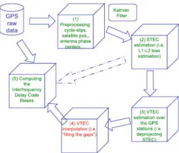
In order to generate the combined VTEC maps several steps are needed and the processes is shown in Figure 1.
Figure 1. Example of data reconstruction procedure as implemented in global VTEC maps (source: UPC (2008)).
Usually, the single ionospheric layer assumption is considered to convert the slant path TEC to vertical TEC with a mapping function. In this work, five analysis centers routinely provide GIMs of vertical TEC using the growing global network of dual frequency GNSS receivers [10]. These are Center for Orbit Determination in Europe (CODE) [11], Jet Propulsion Laboratory (JPL) [12], European Space Agency (ESA) [13], UPC [14], the Energy Mines and Resources Canada (NRCan) [15]. The GIMs VTEC data have a time resolution of 2 hrs and a grid space of 2.5 5 in latitude and longitude, respectively, with errors of several TEC Units [13]. The TEC measurements made by the widely distributed network of ground based GPS receivers are incorporated into the data product. Data gaps, such as those over the oceans where the GPS occultation are not available, are filled in through interpolations and data assimilation techniques [16]. These products are finally validated against the TOPEX TEC data in the case of IGS VTEC. The IGS TEC maps have been recognized and extensively used for studying the properties and variations of the ionosphere [13, 17]. In various studies the vertical total electron content (VTEC) values are estimated by assuming
(1)Ionosphere is distributed homogeneously around local zenith of the receiver;
(2)Ionosphere is stable during at least 5 to 15 minutes; and
(3)The satellite which is closest to the local zenith is chosen.
reference station, in this work TEC was obtained from dual frequency method and the IGS (International GPS Service) TEC map. This GPS station is a non IGS station with in situ data obtained in Rinex file format. IGS TEC map are obtained from IGS data base where TEC map files are in IONEX (Ionosphere Exchange) file format. It is important to underline that the used Rinex file contains data recorded at 30 seconds interval while IONEX file contains data recorded at an interval of 2 hrs. The process of extracting data from RINEX (Receiver Independent Exchange) file was done by using Matlab programming language whereby the RINEX file was obtained from the GPS receiver. The program will analyze and extract the information needed in calculating the TEC from the observation and navigation RINEX file. The result will show the graph of elevation angle, different phase, different delay, slant TEC and vertical TEC versus time.
A dual frequency GPS receiver can measure the difference in ionospheric delays between the and of the GPS frequencies, which are generally assumed to travel along the same path through the ionosphere. Thus, the STEC can be obtained as:
TEC = . −
The line of sight TEC values were converted to VTEC values using a simple mapping function and were associated to an ionospheric pierce point (IPP) latitude and longitude, assuming the ionosphere to be compressed into a thin shell at the peak ionospheric height of 350 km [23].
Figure 2. Ionospheric Single Model (SLM) [11].
Generally by referring to Figure 2, STEC through a given sub ionospheric point is obtained as
!" = !#(cos '()
Where TECs is the value of slant TEC, '(is the difference between 90° and zenith angle (90°− '() [11]
4. Results and Conclusion
In this section we discuss results of comparison of the different data sets with respect to their skill of capturing diurnal, seasonal variabilities of VTEC. The vertical total electron content shows day to day variability due to the regular rotation of the Earth about its own axis following the apparent movement of the Sun.
Ionospheric density is highly depended on the amount of emitted radiation from the Sun. Therefore, the Sun and its activity or relative movement of the Earth orbiting the Sun will mainly result in ionospheric variation. There exists four main classes of regular variations, namely daily, seasonal, 11- year and 27-day variation. Here `regular' implies that the variation could be periodically predicted easily. Besides regular variations, sudden-burst solar activities and character of the geomagnetic field distribution can also lead to special ionospheric phenomena, some of which are diffcult to predict. The ionospheric variation in the tropical area are tightly related to ionospheric storms, travelling ionospheric disturbance, sudden ionospheric disturbance, ionospheric scintillation, and geomagnetic field distribution.
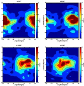
However, the net diurnal change in the quiet day low latitude ionosphere mostly depend on the photoionization production and recombination losses associated with the local solar radiation and the field aligned diffusion of the transported electrons from the equator. In diurnal observation, almost similar diurnal pattern is observed for all different global GPS TEC data. Since the sun is overhead on the equator region, the diurnal peak TEC is observed during 14:00 GMT hrs for different global GPS TEC data between
−60° to 60° longitude, this shows global VTEC corotating with the sun. We can see from contour plots the diurnal TEC variability for every 4 hrs, peak TEC is shifted 60° westwards following the overhead sun.
4.1. Diurnal Variation of VTEC as Captured by Different Data Set
between -180o to 1800 longitudes.
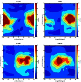
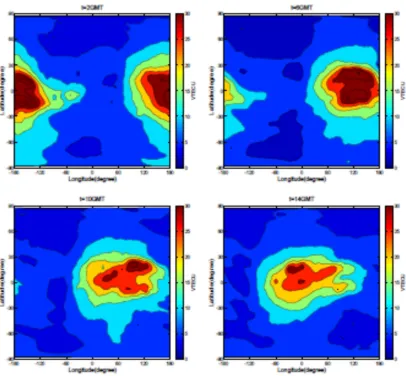
Four hours later (at 6 GMT) the maximum TEC is shifted to between 60° to 180° longitude. At 10 GMT the maximum TEC is observed between 20° to 140 ° longitude. Despite the fact that all the data sets captured diurnal variability, there is some differences on the magnitude of VTEC at different
times of the day in these particular examples. In diurnal observation VTEC from ESA is generally higher than all of them while VTEC from UPC is consistently lower than from all other VTEC data sets. JPL VTEC is the next highest VTEC followed by IGS VTEC and COD VTEC respectively
Figure 3. The Diurnal Variation og IGS VTEC on March 1, 2008 evry four hours.
Figure 5. The Diurnal variation of ESA VTEC on March 1, 2008 every four hours.
Figure 7. The Diurnal variation of UPS VTEC on March 1, 2008 every four hours.
4.2. Seasonal Variation of VTEC as Captured by Different Data Sets
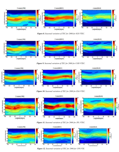
In this study, we can understand that E-season, D-season and J-season variation in VTEC for the year 2008 global GPS TEC data. However, the seasonal VTEC shows relatively maximum VTEC values in JPL and IGS for all seasons.
Seasonal variations are directly related to the Earth orbiting around the Sun. Local winter hemisphere faces away from the Sun results in less received solar radiation, on the contrary, local summer hemisphere results in more received solar radiation. Seasonal variations of the D, E, and F1 layers are mainly determined by the highest angle of the Sun, thus the ionization density of these layers are highest in the summer and lowest in the winter [24]. The F2 layer, however, shows an opposite pattern. Ionization density in F2 layer reaches greatest in the winter and lowest in the summer. The seasonal variation also depends on the temperature, the colder the temperature the less effective recombination rate for molecular N2 and O2. As a result, ionization density presents greatest in the winter [25].
In Figures 8-12, the variation of VTEC during Equinox months, summer solicitice months and winter solicitice
months has been shown. E-season or Equinox months includes March, April, September and October, D-season or Winter solstice months includes January, February, November and December and J-season or summer solstice comprises of May, June, July and August. During the Equinox months, the morning rise and afternoon decay of TEC is sharp compared to solstice seasons. Further the TEC is higher in the E-season (Equinox months) compared to that in the J-season (summer solstice months) and D-season (winter solstice months). As it was noted by [26, 27] during the deep solar minimum (2006 to 2009) the diurnal variation of the VTEC observed over Alexandria is similar to the diurnal variation observed during quiet magnetic period at equatorial latitudes.
Figure 8. Seasonal variation of TEC for 2008 for IGS VTEC.
Figure 9. Seasonal variation of TEC for 2008 for COD VTEC.
Figure 10. Seasonal variation of TEC for 2008 for ESA VTEC.
Figure 11. Seasonal variation of TEC for 2008 for JPL VTEC.
Figure 12. Seasonal variation of TEC for 2008 for UPS VTE.
5. Conclusion
In this study we have used TEC observations for 2008 from globally distributed GPS receivers to describe the TEC variation in the ionosphere at diurnal and seasonal time scales. The gridded global TECs are available from IGS, COD, ESA, JPL
and UPC data centers. The inter comparison between the data sets show that generally ESA VTEC is higher than all of them, followed by JPL, IGS, COD and UPC VTEC respectively.
(summer solstice) in this order for all global GPS TEC data sets. The seasonal VTEC shows relatively maximum VTEC values in JPL and IGS for all seasons. The lowest values of VTEC are observed in UPC relative to other data sets (namely IGS, COD, ESA and JPL) for all seasons.
References
[1] Sizun H., 2005, Radio Wave Propagation for telecommunication Applications, Springer Verlag Berlin Heidelberg, New York.
[2] S. G. Jin, J. Wang, H. Zhang, and W. Zhu, “Real-time monitoring and prediction of Ionosphere Electron Content by means of GPS,” Chin. Astro. Astrophys., vol. 28, pp. 331-337, 2004.
[3] Rishbeth H. and Garriot O. K., 1969. Introduction to Ionospheric Physics, volume 14 of International Geophysics, Academic Press.
[4] McNamara L. F., 1990. The Ionosphere: Communications, Surveillance, and Direction Finding, Krieger publishing company, Malabar, Florida.
[5] Bagiya M. S, Joshi HP, Iyer KN, Aggarwal M, Ravindran S, Pathan BM., 2009. TEC variations during low solar activity period (2005-2007) near the equatorial ionospheric anomaly crest region in India. Ann Geophys 27: 10471057.
[6] Moffett RJ, Hanson WB., 1965. Effect of ionization transport on the equatorial F- region. Nature 206: 705706.
[7] Bradford, W. P. and Spilker, J. J. J., 1996. Global Positioning System: Theory and applications, American Institute of Aeronautics and Astronautics, Vol. I and II Washington DC, USA. [8] Fahmi. A. M, 2015, Comparison of Ionospheric Total Electron Content Measurements with IRI-2012 Model Predictions Over Athens, Iraqi Journal of Science, Vol 56, No. 1A, pp: 246-256. [9] Leonard K., Daniel M., Eleri S. P., Ljiljana R. Cander, Ruth A. Bamford, Anna B., Reinhart L., Sandro M. R, Cathryn N. M., And Paul S. J. Spencer, 2004, Total electron content – A key parameter in propagation: measurement and use in ionospheric imaging, ANNALS OF GEOPHYSICS, SUPPLEMENT TO VOL. 47, N. 2/3.
[10] Ercha, A., D. Zhang, A. J. Ridley, Z. Xiao, and Y. Hao., 2012. A global model: Empirical orthogonal function analysis of total electron content 19992009 data, J. Geophys. Res., 117, A03328, doi: 10.1029/2011JA017238.
[11] Schaer, S.; Markus; R. Gerhard; B. Timon, A. S., 1996. Daily Global Ionosphere Maps based on GPS Carrier Phase Data Routinely produced by the CODE Analysis Center, Proceeding of the IGS Analysis Center Workshop, Silver Spring, Maryland, pp. 181-192, USA.
[12] Ho, C. M., A. J. Mannucci, U. J. Lindqwister, X. Pi, and B. T. Tsurutani, 1996. Global ionosphere perturbations monitored by the worldwide GPS network, Geophys. Res. Lett., 23, 32193222, doi: 10.1029/1996GL02763.
[13] Feltens and schaer, J., and S. Schaer, 1998. IGS products for the ionosphere, IGS Position Paper, in IGS 1998 Analysis Center Workshop: Proceedings, edited by J. M. Dow, J. Kouba, and T. Springer, pp. 225232, EurSpace Oper. Cent., Darmstadt, Germany.
[14] Hernndez-Pajares, M., J. M. Juan, J. Sanz, R. Orus, A. Garcia-Rigo, J. Feltens, A. Komjathy, S. C. Schaer, and A. Krankowski, 2009. The IGS VTEC maps: A reliable source of ionospheric information since 1998, J. Geod., 83, 263275, doi: 10.1007/s00190-008-0266-1.
[15] Gao, Y., P., Heroux, and J. Kouba, 1994. Estimation of GPS receiver and satellite L1/L2 signal delay biases using data from CACS, paper presented at the International Symposium on Kinematic Systems in Geodesy, Geomatics, and Navigation, Univ. of Calgary, Ban, Alberta, Canada.
[16] Mannucci, A. J., B. D. Wilson, D. N. Yuan, C. M. Ho, U. J. Lindqwister, and T. F. Runge, 1998. A global mapping technique for GPS-derived ionospheric total electron content measurements, Radio Sci., 33, 565582.
[17] Wan, W., L. Liu, X. Pi, M.-L. Zhang, B. Ning, J. Xiong, and F. Ding, 2008. Wavenumber-4 patterns of the total electron content over the low latitude ionosphere, Geophys. Res. Lett., 36, L12104, doi: 10.1029/2008GL033755.
[18] Nayir, H., F. Arikan, O. Arikan, and C. B. Erol (2007), Total Electron Content estimation with Reg-Est, J. Geophys. Res., 112, A11313, doi: 10.1029/2007JA012459.
[19] Arikan, F., C. B. Erol, and O. Arikan (2003), Regularized estimation of vertical total electron content from Global Positioning System data, J. Geophys. Res., 109 (A12), 1469, doi: 10.1029/2003JA009605.
[20] Arikan, F., C. B. Erol, and O. Arikan (2004), Regularized estimation of vertical total electron content from GPS data for a desired time period, Radio Sci., 39, RS6012, doi: 10.1029/2004RS003061.
[21] Arikan, F., O. Arikan, and C. B. Erol (2007), Regularized estimation of TEC from GPS data for certain mid-latitude stations and comparison with the IRI model, Adv. in Space Res., 39, 867–874, doi: 10.1016/ j.asr.2007.01.082.
[22] Erol C. B., Arikan F., and Arikan O., 2002a. A new technique for TEC estimation, paper presented at IEEE IGARSS Symp., Toronto, Canada.
[23] Horvath. I and Essex. E. A., 2000. Using observations from the GPS and TOPEX satellites to investigate night-time TEC enhancement at mid-latitudes in the southern hemisphere during a low sunspot number period, Journal of Atmospheric and solar Terrestrial-Physics, Vol. 62, No. 5, pp. 371-391. [24] Integrated Publishing, \Variations In The Ionosphere."
http://www.tpub.com/neets/book10/40h.htm. Retrieved October 19, 2015.
[25] S. Skone, \Lecture Notes of ENGO 633," tech. rep., University of Calgary, 2007.
[26] Shimeis A, Amory-Mazaudier C, Fleury R, Mahrous AM, Hassan AF., 2014, Transient variations of vertical total electron content over some African stations from 2002 to 2012. Advance in Space Research. doi: 10.1016/j.asr.2014.07.038.
![Figure 2. Ionospheric Single Model (SLM) [11].](https://thumb-us.123doks.com/thumbv2/123dok_us/966766.1596069/3.595.55.282.431.660/figure-ionospheric-single-model-slm.webp)