R E S E A R C H Open Access
Affine processes under parameter uncertainty
Tolulope Fadina· Ariel Neufeld · Thorsten Schmidt
Received: 20 June 2018 / Accepted: 23 April 2019 /
© The Author(s). 2019Open AccessThis article is distributed under the terms of the Creative Commons Attribution 4.0 International License (http://creativecommons.org/licenses/by/4.0/), which permits unrestricted use, distribution, and reproduction in any medium, provided you give appropriate credit to the original author(s) and the source, provide a link to the Creative Commons license, and indicate if changes were made.
Abstract We develop a one-dimensional notion of affine processes under parameter
uncertainty, which we callnonlinear affine processes. This is done as follows: given
a setof parameters for the process, we construct a corresponding nonlinear
expec-tation on the path space of continuous processes. By a general dynamic programming principle, we link this nonlinear expectation to a variational form of the Kolmogorov equation, where the generator of a single affine process is replaced by the supremum
over all corresponding generators of affine processes with parameters in. This
non-linear affine process yields a tractable model for Knightian uncertainty, especially for modelling interest rates under ambiguity.
We then develop an appropriate Itˆo formula, the respective term-structure equa-tions, and study the nonlinear versions of the Vasiˇcek and the Cox–Ingersoll–Ross (CIR) model. Thereafter, we introduce the nonlinear Vasiˇcek–CIR model. This model is particularly suitable for modelling interest rates when one does not want to restrict the state space a priori and hence this approach solves the modelling issue arising with negative interest rates.
T. Fadina·T. Schmidt ()
Department of Mathematical Stochastics, University of Freiburg, Ernst-Zermelo Str.1, 79104 Freiburg, Germany
e-mail: [email protected] A. Neufeld
Nanyang Technological University, Division of Mathematical Sciences, Singapore, Singapore T. Schmidt
Freiburg Institute of Advanced Studies (FRIAS), Freiburg im Breisgau, Germany T. Schmidt
Keywords Affine processes·Knightian uncertainty·Riccati equation·Vasiˇcek
model·Cox–Ingersoll–Ross model·Nonlinear Vasiˇcek/CIR model·Heston model
·Itˆo formula·Kolmogorov equation·Fully nonlinear PDE·Semimartingale
1 Introduction
The modelling of a dynamic and unpredictable phenomenon like stock markets or interest rate markets is often approached via choosing an appropriate stochastic model. In many cases, the choice of the model is a delicate and difficult question. In complex dynamic environments like financial markets it is rather the rule than the exception that unforeseen events lead to difficulties with the a priori chosen model and improvements of the model have to be developed and implemented.
A promiment example in this direction is the role of affine short-rate models in the last 20 years: around 2000, the property of the Vasiˇcek model that interest rates can become negative was heavily critizied and the non-negative Cox–Ingersoll–Ross (CIR) model was preferred, the consequences of the financial crises in 2007–2008 leading to negative interest rates in the Euro zone rendered the CIR model no longer applicable and led to a resurgence of the Vasiˇcek model.
This example illustrates the important question of model uncertainty, which is
one of the most important topics in applied sciences and, in particular, plays a prominent role in finance, not only since the financial crisis. The apparent risk of
losses due to model mis-specification, calledmodel risk, fostered the development of
strategies which arerobustagainst model risk, typically leading to nonlinear pricing
rules. These robust strategies play a prominent role in the literature, see Denis and
Martini (2006); Cont (2006); Eberlein et al. (2014); Madan (2016), Acciaio
et al. (2016); Muhle-Karbe and Nutz (2018); Bielecki et al. (2018), and the book
Guyon and 50 Henry-Labord`ere (2013), to name just a few references in this
direction.
A key observation in these works is that the single probability measure used in the classical approaches to specify a model must be replaced by a family of probabil-ity measures (i.e., a full class of models). Such an approach is very natural from the statistical viewpoint: when a model has certain parameters to be estimated, the esti-mators carry statistical uncertainty and one considers confidence intervals instead, corresponding to a family of probability measures. The latter formulation of model
risk is typically referred to asparameter uncertainty, see Avellaneda et al. (1995);
Wilmott and Oztukel (1998), and Fouque and Ren (2014), and is a major motivation
for our research.
Examples in this direction are the notions ofg-Brownian motion andG-Brownian
motion referring to a Brownian motion with drift or volatility uncertainty, see Peng
(1997); Peng (2007a); Peng (2007b) and references therein. Most recently, this theory
has been extended to more general approaches, so-called nonlinear L´evy processes,
see Neufeld and Nutz (2017) and Denk et al. (2017) in this regard.
uncertainty by afamilyof semimartingale laws whose differential characteristics are bounded from above and below by affine functions of the current states. Nonlinear L´evy processes constitute the special case where the bounds do not depend on the state of the process. It seems important to stretch that for affine processes the bounds on drift and volatility are allowed to depend on the state of the process (in an affine way, however). On the contrary, this state dependence leads to a number of addi-tional difficulties and we therefore restrict ourselves to the simplest case, namely, the one-dimensional case without jumps.
It is our aim to provide the appropriate tools for incorporating parameter uncer-tainty in the prominent class of affine models. This naturally leads to a nonlinear version of affine processes and associated nonlinear expectations. After having estab-lished a dynamic programming principle, we establish the connection to the nonlinear Kolmogorov equation. This allows us to study a number of interesting further devel-opments, a nonlinear version of the Itˆo-formula, and nonlinear affine term structure equations.
We also provide a number of examples: in addition to a nonlinear variant of the Black–Scholes model and nonlinear Vasiˇcek and CIR models we also introduce a nonlinear Vasiˇcek–CIR model. In the latter model one can incorporate negative inter-est rates in combination with a CIR-like behaviour, solving the problem raised in many practical applications when the state space needed to be restricted to positive interest rates (see Carver (2012)).
The paper is organized as follows: in Section2, we introduce nonlinear affine
pro-cesses. In Section3we prove that a dynamic programming principle holds. Section4
provides the nonlinear Kolmogorov equation and, as examples, the nonlinear Vasiˇcek
model and the nonlinear CIR model. In Section5, we provide a nonlinear Itˆo
for-mula together with some examples and, in Section6, we study (nonlinear) affine
term structure models. Section7studies the application to model risk and Section8
concludes.
2 Setup
We begin with a short review of continuous affine processes in one dimension. For a detailed exposition we refer to Duffie et al. (2003) and Filipovi´c (2009). Consider the
canonical state space, which is eitherX =RorX =R>0. A (time-homogeneous)
Markov processXwith values in the state spaceX is calledaffineif the conditional
characteristic function ofX is exponentially affine. This means that there existC
-valued functionsφ(t,u)andψ(t,u), respectively, such that
Eeu XT |X t
=eφ(T−t,u)+ψ(T−t,u)Xt
for all complexu∈ {i x :x∈R},0≤t ≤T. The key for our nonlinear formulation
will be a characterization ofXin terms of stochastic differential equations: more
equation
d Xt =
b0+b1Xt
dt+a0+a1X
td Wt, X0=x (1)
where the drift parameterb0+b1Xt and the diffusion parametera0+a1Xt depend
on the current value ofXin an affine way. Here, the processWis a standard
Brow-nian motion. It should be noted that, depending on the state space, not all parameter combinations are possible, but only those combinations which are admissible in the
sense made precise in Theorem 10.2 in Filipovi´c (2009). For our case, this implies
that if on the one sideX =R, we necessarily havea1 =0 anda0>0 and, on the
other side, ifX =R>0, we obtaina0=0,a1>0, andb0>0. In addition, the
coef-ficientsφandψsolve ODEs (classified as Riccati equations), which is the essence
for the high degree of tractability of affine processes in the sense that explicit calcu-lations are possible or efficient numerical methods are obtainable; see Duffie et al. (2003); Filipovi´c (2009) for details and applications in this regard.
2.1 Nonlinear affine processes
In this section, we introduce the necessary tools for defining affine processes under
parameter uncertainty. To this end, fix a final time horizonT > 0 and let =
C([0,T])be the canonical space of continuous, one-dimensional paths. We endow
with the topology of uniform convergence and denote byF its Borelσ-field. Let
Xbe the canonical processXt(ω)=ωt, and letF=(Ft)t≥0withFt =σ(Xs,0≤
s≤t)be the (raw) filtration generated byX.
As we are interested in semimartingale laws on, we begin by denoting byP()
the Polish space of all probability measures on equipped with the topology of
weak convergence1. The processXwill be called a (continuous)P-F-semimartingale,
for P ∈ P(), if there exist processes B = BP and M = MP such that X =
X0+B+M, whereBhas continuous paths of (locally) finite variationP-a.s.,M is
a continuousP-F-local martingale andB0=M0=0.
It will be important in the following that, by Proposition (2.2) in Neufeld and
Nutz (2014),Xis aP-F-semimartingale if and only if it is aP-semimartingale with
respect to the right-continuous filtration F+ = (Ft+)t≥0 or with respect to the
usual augmentationF+P; hereFt+= ∩s>tFs. Hence, in the following, we consider
semimartingales with respect to the raw filtrationF.
TheP-F-characteristics of a continuous semimartingale X = X0+BP+MP in
the above representation is the pairBP,C, whereC = MP. The non-negative
processCdoes not depend onP, as the quadratic variation is a path property2. For
the following, we will focus on semimartingales where the semimartingale
character-istics are absolutely continuous (a.c.), i.e., there exist predictable processesβP and
1The weak topology is the topology induced by the bounded continuous functions on. Then,P()is a
separable metric space and we denote the associated Borelσ-field byB(P()).
2This is becauseCcan be constructed as a single process not depending onP; that is, two measures under
α≥0, such that
BP= ·
0β P
s ds, C=
·
0α
sds. (2)
A probability measure P ∈ P()is called asemimartingale lawforX, ifXis a
P-F-semimartingale. We denote by
Pacsem= {P∈P()|Xis aP-F-semimartingale with a.c. characteristics}
the set of all semimartingale laws ofXwhich have absolutely continuous
characteris-tics. In the following, we denote byβP, α, as in (2), the differential characteristics ofXunder P∈Pacsem.
Our main goal is to allow for a specific version ofmodel riskin the sense that there
is uncertainty on the parameter vectorθ =b0,b1,a0,a1of the affine process. We
assume that there is additional information on bounds on the parameter vectorθand
denote these finite bounds bybi,b¯i,ai,a¯i,i = 0,1, respectively. This leads to the compact set
=b0,b¯0×b1,b¯1×a0,a¯0×a1,a¯1⊂R2×R2≥0. (3)
We are interested in the intervals generated by the associated affine functions. In this regard, let B := b0,b¯0×b1,b¯1and A := a0,a¯0×a1,a¯1. Moreover, we denote fora∈R2,a:=(a0,a1)and similarly forb∈R2. Furthermore, let
b∗(x):=
b0+b1x:b∈ B
,
a∗(x):=
a0+a1x+:a∈ A
(4)
for x ∈ R denote the associated set-valued functions. As the state space will, in
general, beR, we have to ensure non-negativity of the quadratic variation which is
achieved using(·)+:=max{·,0}in the definition ofa∗. Due to the nice structure of
, the sets are always intervals: indeed,
b∗(x)=b0+b11{x≥0}+ ¯b11{x<0}
x,b¯0+b¯11{x≥0}+b11{x<0}
x,
a∗(x)= [a0+a1x+,a¯0+ ¯a1x+].
(5)
Clearly, it is possible to consider a more general, however, this is not our focus
here.
Definition 1Letbe a set as in(3)with associated a∗, b∗as in(4), let t∈ [0,T], and let P∈ Pacsembe a semimartingale law. We call P affine-dominated on(t,T]by , ifβP, αsatisfy
βP
s ∈b∗(Xs), and αs ∈a∗(Xs), (6)
for d P⊗dt-almost all(ω,s)∈×(t,T]. If t =0, we call P affine-dominated by.
An affine process can be uniquely characterized by its transition probabilities. We will make use of this fact for characterizing affine processes under model uncertainty.
Moreover, we denote byOthe considered state space, which will be eitherR,R≥0,
Definition 2Letbe a set as in(3)with associated a∗, b∗as in(4). A nonlinear affine process starting at x∈Ois the family of semimartingale laws P ∈Pacsem, such that
(i) P(X0=x)=1,
(ii) P is affine-dominated by.
As explained in the introduction, parameter uncertainty is represented by a family of models replacing the single model in the approaches without uncertainty:
accord-ing to Definition2, the affine process under parameter uncertainty is represented by
afamilyof semimartingale laws instead of a single one. We denote the
semimartin-gale lawsP ∈ Pacsem, satisfying P(X0 = x)=1 and being affine-dominated by
byA(x, ). Intuitively, this corresponds to a nonlinear affine process starting inx.
It is well known that the state spaceOneeds to be chosen in correspondence with
the choice of: indeed, the squared Bessel process is an affine process with state
spaceR>0 (see, for example, Karatzas and Shreve (1988), Prop. 3.22 of Chap. 3)
and the setA(x, )will be empty forx < 0. To exclude additional difficulties in
this direction, we call a family of nonlinear affine processes(A(x, ))x∈Owith state spaceOproper, if eithera0>0 holds, ora0= ¯a0=0 andb0≥a¯1/2>0.
It is clear that in the case withO = Rthe assumptiona0 > 0 is sufficient for
reaching the full state space. The case with non-negative state spaces is more delicate.
We concentrate on the caseO =R>0. The following proposition gives a sufficient
condition in this regard. Moreover, it shows that the nonlinear affine process does not reach zero, in the sense that the event of reaching 0 has zero probability under all P∈A(x, ).
Proposition 1Let x>0, and assume that a0= ¯a0=0and b0≥a¯1/
2>0. Then, for any P∈A(x, ), it holds that
P(Xt >0, 0≤t≤T)=1.
ProofLetP ∈A(x, ), denote byβPandαthe associated processes from Eq.2,
and denote byMPtheP-local martingale part of theP-semimartingaleX. Moreover,
for anyc≥0 define
τc :=inf{t≥0: Xt =c}.
We need to show for any timeT > 0 that P[τ0 ≤ T] = 0. To that end, fix an
arbitraryT >0. We adopt the method in Gikhman (2011) to our setting: letεsuch
that 0< ε <x. Note that by continuity of the paths ofX, we have that X ≥ ε >0 on[[0, τε]]. Moreover, by assumption,
m:= 2b 0− ¯a1
¯
Itˆo’s formula yields for anyt ≥0 that
(Xτε∧t)−m=(X0)−m−
τε∧t
0
m Xs−(m+1)βsPds+1 2
τε∧t
0
m(m+1)Xs−(m+2)αsds
− τε∧t 0
m Xs−(m+1)d MsP.
Define the processesMandM˜ by
Mt = − t
0
m X−s(m+1)d MsP, t ≥0,
˜ Mt =
t
0 (
Xτε∧s)−(m+1)d MsP, t ≥0.
Clearly, bothM and M˜ are local martingales and M = −mM˜ on[[0, τε]]. We now
show thatM˜ is a true martingale. By the Burkholder–Davis–Gundy inequality, since
X ≥εon[[0, τε]], we obtain that
E
sup 0≤s≤T| ˜
Ms|
≤C E
T
0
Xτ−ε2∧(sm+1)ατε∧sds
1/2
≤C E
¯ a1
T
0
X−τε2∧(sm+1)+1ds
1/2
≤C(a¯1ε−2(m+1)+1T)1/2<∞
and henceM˜ is indeed a martingale. Therefore,M is a true martingale on[[0, τε]].
Next, sinceP∈A(x, )andm>0, we obtain the estimate
X−τεm∧t
≤x−m−
τε∧t
0
m X−s(m+1)
b0+b1Xs
ds
+1
2
τε∧t
0
m(m+1)Xs−(m+2)a¯1Xsds+Mτε∧t
=x−m−mb1
τε∧t
0
X−smds+
τε∧t
0
m(m+1)a¯1
2 −mb
0
X−s(m+1)ds+Mτε∧t.
Taking expectations and using thatX ≥ε >0 on[[0, τε]]yields, in view of (7), for allt ≥0 that
E(Xτε∧t)−m
≤x−m−mb1 τε∧t
0
E(Xs)−m
ds ≤x−m+m|b1| τε∧t
0
E(Xs)−m
ds (8)
Moreover, asX≥ε >0 on[[0, τε]], we obtain that
m|b1| τε∧t
0
E(Xs)−m
ds=m|b1| t
0
1{s≤τ}E
(Xτε∧s)−m
ds≤m|b1| t
0
E(Xτε∧s)−m
ds.
This together with (8) yields for anyt≥0 that
EXτε∧t
−m
≤x−m+m|b1| t
0
E(Xτε∧s)−m
By means of Gronwall’s inequality, we obtain for allt ≥0 that
EXt∧τε
−m
≤x−mem|b1|t. (9)
In particular, we obtain by Chebyshev’s inequality for our fixed timeT >0 that
P(τε <T)=P(Xτε∧T ≤ε)= PXτε∧T−m ≥ε−m
≤εm
E(Xτε∧T)−m.
Inserting (9) and lettingεtend to zero yields the claim. The proof of Proposition1is
thus complete.
3 Dynamic programming
One of the key insights for Markov processes is the deep link between Markov
processes and their expectations to partial differential equations given by the
Kol-mogorov equation. In this section, we generalize this relation to the case with parameter uncertainty, i.e., we develop the relation of the nonlinear affine process to a nonlinear version of the Kolmogorov equation. The path we detail in this section
uses dynamic programming and the results obtained in Nutz and van Handel (2013)
and El Karoui N and Tan (2013a). The key to dynamic programming is a certain
sta-bility property under conditioning and pasting. As the nonlinear affine processes we
considered up to now always start from timet = 0, we introduce the appropriate
conditional formulations first.
For the remainder of the section, fixas in (3) with associateda∗andb∗ as in
(4). Denote byA(t,x, )the semimartingale lawsP∈Pacsem, such that
(i) P(Xt =x)=1, and
(ii) Pis affine-dominated on(t,T]by.
The following result yields measurability of the nonlinear affine process starting attinω(t).
Lemma 1The set(ω,t,P)∈× [0,T] ×P()P∈A(t, ω(t), )is Borel.
ProofBy Theorem 2.6 in Neufeld and Nutz (2014), the setPacsemis Borel, which proves that
(ω,t,P)∈× [0,T] ×PacsemP(Xt =ω(t))=1
is Borel. Moreover, Theorem 2.6 in Neufeld and Nutz (2014), also grants the
existence of a Borel-measurable map
such that(βP, α) are the differential characteristics of X under P. Therefore, we obtain the Borel measurability of the set
G:=
(ω,t,P,ω,s)∈× [0,T] ×Pacsem×× [0,T]
s>t,
P(Xt =ω(t))=1,
βP
s (ω), αs(ω)
∈b∗(Xs(ω))×a∗(Xs(ω))
.
Applying Fubini’s theorem yields the Borel measurability of the set
G:=
(ω,t,P,ω)∈× [0,T] ×Pacsem× T
0
1G(ω,t,P,ω,s)1(t,T](s)ds=T−t
.
Now, observe that
(ω,t,P)∈× [0,T] ×P()P ∈A(t, ω(t), ) = (ω,t,P)∈× [0,T] ×Psemac EP[1G(ω,t,P,·)] =1
.
The right side is Borel measurable due to a monotone class argument as in ((Neufeld
and Nutz2014), Lemma 3.1).
Lemma 2Fix(x,t)∈R× [0,T],P ∈ A(t,x, )and a stopping timeτ taking values in[t,T].
(i) There exists a family of conditional probabilities(Pω)ω∈of P with respect to
Fτ such that Pω∈A(τ(ω), ωτ(ω), )for P-a.e.ω∈.
(ii) Assume that there exists a family of probability measures(Qω)ω∈such that Qω ∈ A(τ(ω), ωτ(ω), )for P-a.e.ω ∈ , and the mapω → Qω isFτ measurable. Then, the probability measure P⊗Q defined by
P⊗Q(·)=
Qω(·)P(dω)
is an element ofA(t,x, ).
ProofThis follows directly from ((Neufeld and Nutz2017), Theorem 2.1), see
also ((Guo et al.2017), Lemma 4.6).
Now, fix a Borel-measurable functionψ :O →Rand define the value function
v: [0,T] ×O →Rby
v(t,x):= sup P∈A(t,x,)
EP[ψ(XT)].
Using the above results, we obtain the following dynamic programming principle.
Proposition 2Consider a proper family of nonlinear affine processes with state spaceO. For any(t,x)∈ [0,T] ×Oand any stopping timeτtaking values in[t,T], we obtain
v(t,x)= sup P∈A(t,x,)
ProofThe result follows from Theorem 2.1 in El Karoui and Tan (2013b) (with
Pt,x =A(t,x, )in the notation of El Karoui and Tan (2013b)) by noting that
ana-lyticity is implied by measurability as shown in Lemma1and the required stability
assumptions have been shown in Lemma2.
3.1 Continuity of the value function
In the following, we show the continuity of the value functionv(t,x). To this end,
introduce the constant
K= |b0| + |b1| + | ¯b0| + | ¯b1| + ¯a0+ ¯a1, (10)
which is finite by Assumption (3). The following inequality is the cornerstone of the
results in this section.
Lemma 3Consider a proper family of nonlinear affine processes with state space
Oand let q ≥1. There exists an0< ε≡ε(q) <1such that for all0<h≤ε, all t∈ [0,T −h]and all x ∈O, we have
sup P∈A(t,x,)
EP
sup 0≤s≤h|
Xt+s−x|q
≤C
hq+hq/2
for some constant C=C(x,q) >0which may depend on x, but is independent of h and t.
ProofLet q ∈ [1,∞). Consider P ∈ A(t,x, ) and denote by Xs = x + BP
s +MsP,s ≥ t, the semimartingale representation of X with predictable
finite-variation partBPand local martingaleMP. In the following, we will repeatedly use
the elementary inequality that
(a1+a2)q ≤2q−1(aq1+a2q) (11)
and denotecq :=2q−1.
The Burkholder–Davis–Gundy (BDG) inequality (see Theorem 4.1 in Revuz and
Yor (1999)) together with Jensen’s inequality and (11) yields for anyh∈ [0,T −t]
that
EP
sup 0≤s≤h|
Xt+s −x|q
≤cqEP
sup 0≤s≤h
MtP+sq
+cqEP
sup 0≤s≤h
BtP+sq
≤cqCqEP
t+h
t α
udu
q/2
+cqEP
t+h
t
βP
udu
q
.
(12)
Note that the constantCq≥1 from the BDG inequality does depend onqonly.
LetK:= 1+K, whereKis the constant defined in (10). Choose any 0 < ε =
ε(q) <1 small enough such that it satisfies
1−c3qCqKq
εq+εq/2>
Let us verify that such a fixedεsatisfies the desired property: by the very definition
ofP ∈ A(t,x, ), we have on[t,t +h] that bothαand|βP|are bounded from
above byK+Ksup0≤s≤h|Xt+s| ≥1 since they are affine dominated. This, together with Jensen’s inequality, yields that
EP
t+h
t α udu
q/2
≤hq/2EP ⎡ ⎣
K+K sup
0≤s≤h|
Xt+s| q/2⎤
⎦
≤hq/2EP
K+K sup
0≤s≤h|
Xt+s| q
≤hq/2cq
Kq+KqEP
sup
0≤s≤h|
Xt+s| q
≤hq/2c2q
Kq+Kq|x|q+KqEP
sup
0≤s≤h|
Xt+s−x| q
.
In a similar way, we obtain
EP
t+h
t |β P u|du
q
≤hqEP
K+K sup
0≤s≤h|
Xt+s| q
≤hqcq2
Kq+Kq|
x|q+KqEP
sup
0≤s≤h|
Xt+s−x| q
.
Inserting these inequalities into (12), considering h ≤ ε, and noting thatC˜q ≥ 1
implies that
EP
sup
0≤s≤h|
Xt+s−x|q
≤c3qCqKq
hq/2+hqEP
sup
0≤s≤h|
Xt+s−x|q
+cq3CqKq(1+ |x|q)
hq/2+hq
≤c3qCqKq
εq/2+εq
EP
sup
0≤s≤h|
Xt+s−x|q
+cq3CqKq(1+ |x|q)
hq/2+hq
.
(14)
Sinceh≤εand we chose 0< ε <1 such that (13) holds, we obtain for the constant
C := c
3
qCqKq(1+|x|q) 1−c3
qCqKq(εq/2+εq) >0, being independent oft,h,P, that
EP
sup 0≤s≤h|
Xt+s −x|q
≤C hq/2+hq.
AsP ∈A(t,x, )was chosen arbitrarily, the claim is proven.
Lemma 4Consider a proper family of nonlinear affine processes with state space
Oand letψ:O →Rbe Lipschitz continuous with Lipschitz-constant Lψ. Then, the value function
v(t,x):= sup P∈A(t,x,)
EP[ψ(XT)]
is jointly continuous. In particular,v(t,·)is Lipschitz continuous with constant Lψ andv(·,x)is locally1/2-H¨older continuous.
ProofFor the Lipschitz-continuity ofv(t,·), observe that for anyt |v(t,x)−v(t,y)| ≤ sup
P∈A(t,x,)
EP[|ψ(XT)−ψ(y−x+XT)|]≤ Lψ|y−x|.
For the locally 1/2-H¨older continuity, lett ∈ [0,T)and 0 ≤ u ≤ T −t be small
enough. Then, the dynamic programming principle derived in Proposition 2, the
Lipschitz continuity ofv(t,·), and Lemma3yield
|v(t,x)−v(t+u,x)| =
P∈Asup(t,x,)
EPv(t+u,Xt+u)−v(t+u,x)
≤ Lψ sup
P∈A(t,x,)
EP|Xt+u−x|
≤ LψC(x,1)u1/2+u
with constantC(x,1)from Lemma3. Finally, consider a sequence(tn,xn) converg-ing to(t,x). Then,
|v(tn,xn)−v(t,x)| ≤ |v(tn,xn)−v(tn,x)| + |v(tn,x)−v(t,x)| ≤Lψ|xn−x| +LψC(x,1)
|tn−t|1/2+ |tn−t|
.
Lettingngo to infinity yields the result.
4 The Kolmogorov equation
In this section, we provide the link between the nonlinear affine process and the asso-ciated nonlinear Kolmogorov equation. More precisely, we relate the nonlinear affine process to a (fully) nonlinear partial differential equation (PDE). This is achieved by a probabilistic construction involving an optimal control problem on the canonical space of continuous paths where the controls are laws of affine-dominated
semi-martingales. To this end, note that the affine processX given in Eq.1is uniquely
characterized by its infinitesimal generator,
Lθ f(x)=
b0+b1x
∂xf(x)+ 1 2
a0+a1x+
∂x xf(x). (15)
This is equivalent to f(Xt)− f(x)−0tLθf(Xs)ds, 0 ≤ t ≤ T solving the
Consider the state spaceO which will be eitherR,R≥0orR>0. Fixψ:O → R and consider the fully nonlinear PDE
−∂tv(t,x)−G(x, ∂xv(t,x), ∂x xv(t,x))=0 on[0,T)×O,
v(T,x)=ψ(x) x∈O, (16)
whereG:O×R×R→Ris defined by
G(x,p,q):= sup
(b0,b1,a0,a1)∈
(b0+b1x)p+1 2(a
0+ a1x+)q
. (17)
The function−Gsatisfies the degenerate ellipticity condition and asis compact,
it is also continuous. Observe that the PDE defined in (16) can be seen as nonlinear
affine PDE, since forθ:=b0,b1,a0,a1it is of the form
−∂tv(t,x)−supθ∈Lθv(t,x)=0 on[0,T)×O, v(T,x)=ψ(x) x∈O.
We writeC2b,3([0,T)×O)for the set of functions on[0,T)×Ohaving bounded
continuous derivatives up to the second and third order intandx, respectively. An
upper semicontinuous functionuon[0,T)×Owill be called a viscosity subsolution
of (16) ifu(T,·)≤ψ(·)and
−∂tϕ(t,x)−G
x,Dxϕ(t,x),D2x xϕ(t,x)
≤0
wheneverϕ ∈ C2b,3([0,T)×O)is such thatϕ ≥ uon[0,T)×O andϕ(t,x) =
u(t,x). The definition of a viscosity supersolution is obtained by reversing the
inequalities and the semicontinuity. Finally, a continuous function is a viscosity solution if it is both a sub- and a supersolution.
We obtain a stochastic representation for the nonlinear affine PDE (16).
Theorem 1Consider a proper family of nonlinear affine processes with state spaceOand letψ :O→Rbe Lipschitz continuous. Then,
v(t,x):= sup P∈A(t,x,)
EP[ψ(XT)], x∈O
is a viscosity solution of the nonlinear PDE in(16).
ProofThe proof essentially follows the well-known standard arguments in
stochastic control, see e.g., the proof of ((Neufeld and Nutz2017), Proposition 5.4).
By Lemma4,v(t,x)is continuous on[0,T)×R, and we havev(T,x)=ψ(x)by
the definition ofv. We show thatvis a viscosity subsolution of the nonlinear affine
PDE defined in (16); the supersolution property is proved similarly. We remark that
in the subsequent lines within this proof,C > 0 is a constant whose values may
change from line to line.
Let(t,x)∈ [0,T)×Rand letϕ ∈ Cb2,3[0,T)×Rdbe such thatϕ ≥ v and
we have for any 0<u<T −tthat
0= sup
P∈A(t,x,)
EPv(t+u,Xt+u)−v(t,x)
≤ sup
P∈A(t,x,)
EPϕ(t+u,Xt+u)−ϕ(t,x).
(18)
Fix anyP ∈A(t,x, ), denote as above byβP, αthe differential characteristics of
the continuous semimartingaleXunderP, and denote byMPtheP-local martingale
part of theP-semimartingaleX. Then, Itˆo’s formula yields
ϕ(t+u,Xt+u)−ϕ(t,x)= u
0 ∂
tϕ(t+s,Xt+s)ds+ u
0 ∂
xϕ(t+s,Xt+s)d MtP+s
+ u
0 ∂
xϕ(t+s,Xt+s)βtP+sds+ 1 2
u
0 ∂
x xϕ(t+s,Xt+s)αt+sds. (19) Asϕ ∈Cb2,3([0,T)×R), ∂xϕis uniformly bounded, thus by Remark1, we see that
for small enough 0< u < T −t the local martingale part in (19) is in fact a true
martingale, starting at 0. In particular, its expectation vanishes. The next step is to estimate the expectation of the other terms. In this regard, note that
EP u
0 ∂
xϕ(t+s,Xt+s)βtP+sds
≤ u
0 EP
|∂xϕ(t+s,Xt+s)−∂xϕ(t,x)|βtP+s+∂xϕ(t,x)βtP+s
ds.
(20)
Sinceϕ∈Cb2,3,∂xϕis Lipschitz. Hence, we obtain with the constantKfrom Eq.10
together with Lemma3that for small enoughu,
u
0
EP|∂xϕ(t+s,Xt+s)−∂xϕ(t,x)| ·βtP+s
ds ≤ C u 0 EP
s+ sup
0≤v≤u|
Xt+v−x|
·βP
t+s
ds ≤ C u 0 EP
s+ sup
0≤v≤u|
Xt+v−x| K+K sup 0≤v≤u|
Xt+v|
ds ≤ C u 0 EP
s+ sup
0≤v≤u|
Xt+v−x| K+K|x| +K sup 0≤v≤u|
Xt+v−x|
ds
≤ Cu3+u5/2+u2+u3/2
.
(21) Inserting (21) into (20) yields
EP u
0 ∂
xϕ(t+s,Xt+s)βtP+sds
≤ u
0
EP∂xϕ(t,x) βtP+s
The same argument applied to∂x xϕleads to
EP u
0 ∂
x xϕ(t+s,Xt+s) αt+sds
≤ u
0
EP∂x xϕ(t,x) αt+s
ds+Cu3+u5/2+u2+u3/2. (23) Moreover, by a similar calculation, we have
EP u
0 ∂
tϕ(t+s,Xt+s)ds
≤ u
0 ∂
tϕ(t,x)ds+ u
0
EP|∂tϕ(t+s,Xt+s)−∂tϕ(t,x)|
ds
≤ u
0 ∂
tϕ(t,x)ds+C u
0 EP
s+ sup
0≤v≤u|
Xt+v−x|
ds
≤ u
0 ∂
tϕ(t,x)ds+C
u2+u3/2
.
(24)
As above, we write θ := b0,b1,a0,a1 for an element in . Then, by taking
expectations in (19) and using (20)–(24) yields
EPϕ(t+u,Xt+u)−ϕ(t,x)
≤Cu3+u5/2+u2+u3/2
+ u
0
∂tϕ(t,x)+EP
∂xϕ(t,x) βtP+s+∂x xϕ(t,x) αt+s
ds
≤C
u3+u5/2+u2+u3/2
+u∂tϕ(t,x)
+ u 0 EP sup θ∈
(b0+b1Xt+s) ∂xϕ(t,x)+ 1 2
a0+a1X+t+s∂x xϕ(t,x) . (25) Here, the supremum turns out to beG(Xt+s, ∂xϕ(t,x), ∂x xϕ(t,x)). Note that by the
very definition ofG,
G(Xt+s,p,q)≤G(x,p,q)+sup
θ∈
|b1| |Xt+s−x| |p| + |a1| |Xt+s −x| |q|
.
Therefore, by using that ϕ ∈ Cb2,3, the definition of the constantK in (10), and
Lemma3, we have
u
0
EPG(Xt+s, ∂xϕ(t,x), ∂x xϕ(t,x))}
ds
≤ uG(x, ∂xϕ(t,x), ∂x xϕ(t,x))+uCKEP|Xt+s−x| ≤ uG(x, ∂xϕ(t,x), ∂x xϕ(t,x))+CK
u2+u3/2.
Combining (25)–(26) yields
EPϕ(t+u,Xt+u)−ϕ(t,x)≤ u∂tϕ(t,x)+uG(x, ∂xϕ(t,x), ∂x xϕ(t,x)) +Cu3+u5/2+u2+u3/2. (27)
for some constantC >0 which is independent ofP. As the choice ofP ∈A(t,x, )
was arbitrary, we deduce from (18) that
0≤ sup
P∈A(t,x,)
EPϕ(t+u,Xt+u)−ϕ(t,x)
≤u∂tϕ(t,x)+uG(x, ∂xϕ(t,x), ∂x xϕ(t,x))+C
u3+u5/2+u2+u3/2. (28)
By dividing first in (28) by−uand then lettingugo to zero, we obtain that
−∂tϕ(t,x)−G(x, ∂xϕ(t,x), ∂x xϕ(t,x))≤0,
which proves thatvis indeed a viscosity subsolution as desired.
4.1 Uniqueness
Uniqueness in our framework is not covered by standard arguments as in Fleming
and Soner (2006) or Crandall et al. (1992), since the diffusion coefficient does not
satisfy a global Lipschitz condition. This is a well-known difficulty already discussed
in Feller (1951). To overcome this, we have to distinguish the two cases where the
state space is eitherRorR>0.
We begin with the general case which covers the nonlinear Vasiˇcek–CIR model
discussed in detail in Section6.1. In this case we do not decide a priori whether a
Vasiˇcek or a Cox–Ingersoll–Ross (CIR) model takes place and therefore consider the
full spaceRas state space. To achieve this, we assume throughout a non-vanishing
volatility, i.e.,a0>0. When the process reaches zero from above, this avoids that a
deterministic behaviour onR<0takes place and that singularities arise. On the other
side, we do not need any assumptions ona1.
Proposition 3Assume that a0>0and letO =R. Then, for any given continuous and bounded functionψ :R→R, the nonlinear PDE introduced in(16)–(17)admits at most one viscosity solutionv(t,x)on[0,T] ×Rsatisfying the terminal conditions
v(T,x)=ψ(x), x∈R.
ProofUniqueness in this case follows by the observation that the coefficients are
Lipschitz oncea0 > 0. Indeed, then following the standard procedure detailed in
section V.9 in Fleming and Soner (2006) allows to extend the uniqueness results from
Corollary V.8.1 therein to an unbounded domain as considered here.
On the other side, if we consider the case whereR>0is the state space, we will
necessarily requirea0 = ¯a0 = 0.Then, the (bounds on the) diffusion coefficient
be applied. To the best of our knowledge, only Costantini et al. (2012) and Amadori
(2007) treat this setting, though we apply the techniques from the second article.
In this regard, let
h(x)= ⎧ ⎨ ⎩
maxlog1(x),1 =0 maxx1,1
otherwise. (29)
Proposition 4Assume that a0 = ¯a0 = 0,b0 ≥ a¯1/
2 > 0, letO = R>0, and consider a Lipschitz-continuousψ:O→R.
(i) Then,(16)–(17)has a one and only one viscosity solution v on [0,T] ×O satisfying
sup
(t,x)∈[0,T]×O
|v(t,x)|
1+x <∞. (30)
(ii) Let=2b0/a¯1−1>0and suppose that there isρ, ρ>0and∈ [0, )such that |1ψ(+|xx)|| is bounded on(0,∞)and
x→ |ψ(x)|
h(x) (31)
is bounded from above, respectively, in the set(ρ,∞)and(0, ρ). Then, (16)– (17) has one and only one viscosity solutionv(t,x)on[0,T] ×Osatisfying
lim sup x→∞
sup t∈[0,T]
|v(t,x)|
x2 =0, xlim→0 sup t∈[0,T]
|v(t,x)|
h(x) =0. (32)
ProofPositivity follows readily from Proposition1. This will allow to treat the
nonlinear PDE in (16)–(17) on the state spaceO =R>0. The key for uniqueness is
that on compact subsets ofR>0the square-rootisLipschitz continuous.
To begin with, note that existence of a solution under the Lipschitz property of
ψfollows from Theorem1. Furthermore, Theorem 4 in Amadori (2007) yields the
desired uniqueness in our case. We recall this result together with its assumptions in
Appendix2. The claim then follows from Theorem2.
Remark 2Already, the results in the case without uncertainty in Costantini et al. (2012) show that these results do not generalize toR≥0, because then the Lipschitz property on compact subsets which is crucially used in the proof will no longer be satisfied. Moreover, Example 1 in Amadori (2007) shows that the condition b0 ≥ ¯
a1/
2>0is indeed necessary for uniqueness.
4.2 The nonlinear Vasiˇcek model
The first example of an affine model is the so-called Vasiˇcek model, see, for example,
Filipovi´c (2009). It is a Gaussian Ornstein–Uhlenbeck process and is obtained as the
strong solution of the SDE in Eq.1by consideringa1 = 0. Introducing parameter
uncertainty, we arrive at the nonlinear affine process witha1,a¯1 = {0}. We call
this case thenonlinear Vasiˇcek model.
While in the case with no parameter uncertainty, this model can be characterized efficiently by its Fourier transforms and the associated Riccati equation, this is no
longer possible here (except for the special case whereb1= ¯b1, see Remark4below)
and one has to rely on numerical techniques. In one dimension, this does not pose a
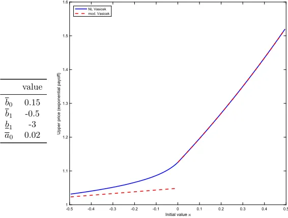
problem, see, for example, Heider (2010). To illustrate this, we solve the equation for
the simplest payoff, f(x)=ex. The result is shown in Fig.1.
This example combines and encompasses the following two well-known nonlinear
processes:g-Brownian motion and G-Brownian motion, see Peng (1997) and Peng
(2007a), for example, and Neufeld and Nutz (2017) for the case with jumps. In the following, we will also elaborate on the case where explicit solutions can be obtained,
see Proposition5and Remark4.
4.3 The nonlinear CIR model
While the Gaussianity of the Vasiˇcek model immediately implies that the pro-cess becomes negative with positive probability, this is inappropriate for various
Fig. 1 This figure shows the solution of the nonlinear Kolmogorov equation for the nonlinear Vasiˇcek-model with boundary condition f(x) =ex. The dashed line shows the solutions for the Vasiˇcek model with parameter-set(b0,b1,a0)(onR<0) and(b0,b1,a0)(onR≥0) and illustrate the nonlinearity in the
applications, e.g., in credit risk. There, the considered affine process models an inten-sity, which by definition has to be non-negative. Also, positive interest rates were a requirement before the recent crises in 2008–2010. The Cox–Ingersoll–Ross (CIR)
model serves as an affine model with state spaceR≥0 and therefore satisfies these
needs. It is obtained by choosinga0=0 anda1>0 in the SDE in (1).
The CIR model under parameter uncertainty, which we call the nonlinear CIR
model, is obtained by considering the state spaceO =R>0and assuming thata0=
¯
a0 = 0,b0 ≥ a¯1/2 > 0. It is remarkable how far-reaching the positivity ofX will be: indeed, a first look at the nonlinear Kolmogorov equation already reveals that
for increasing and convex functions the supremum in Eq.17will be attained by the
upper bounds of the coefficients.
The Fourier-transform which is lacking monotonicity (asei ux does) turns out to
lose tractability in the nonlinear case considered here. The Laplace transform does not suffer from this problem and we show in the following that in important special cases it can be computed explicitly. However, inversion techniques can no longer be applied in the nonlinear setting and the Laplace transform merely serves as a prime example of an increasing convex function for which the nonlinear expectations can be computed explicitly in special cases (and for decreasing concave functions of course).
Remark 3In principle, the nonlinear CIR model can be extended to the whole space, i.e., choosingO = Ris possible, since in Eq. 4, negative values pose no problem. For x negative, the dynamics of the model have no diffusive part and only move through the drift (which of course can still be stochastic). This could happen with a positive (upper) mean-reversion level and by starting from a negative value.
We begin with a general result for affine processes which classifies when the classical representation via Riccati equations still holds.
Recall from (5), that b∗(x)and a∗(x) are actually intervals. Define the upper
bound ofa∗(x)by
¯
a(x):= ¯a0+ ¯a1x+. (33)
Note that the upper bound ofb∗(x)is given by
¯
b(x):= ¯b0+b1x1{x<0}+ ¯b1x1{x≥0}. (34)
LettingB¯1,x =b11{x<0}+ ¯b11{x≥0},we obtain thatb¯(x)= ¯b0+ ¯B1,xx.Note that forx= ywe may no longer have thatb¯(x)= ¯b0+ ¯B1,yx.
Proposition 5Consider a nonlinear affine processA(x, )and assume that for all P∈A(x, )
βP
t ≤ ¯b0+ ¯B1,xXt, (35)
d P⊗dt-almost everywhere for0≤t ≤T . Moreover, assume either that a1= ¯a1= 0or that for all P∈A(x, ), Xt ≥0P⊗dt-a.e. If there exists aP¯ ∈A(x, )and aP-¯ F-Brownian motion W such that the canonical process under P is the unique¯ strong solution of
d Xt =(b¯0+ ¯B1,xXt)dt+
¯
then, for all u≥0and0≤t ≤T ,
sup P∈A(x,)
EPeu Xt=exp(φ(t,u)+ψ(t,u)x) ,
whereφ, ψsolve the Riccati equations
∂tφ(t,u)= 1 2a¯
0ψ(
t,u)2+ ¯b0ψ(t,u), φ(0,u)=0 (37)
∂tψ(t,u)= 1 2a¯
1ψ(
t,u)2+ ¯B1,xψ(t,u), ψ(0,u)=u. (38)
This result is obtained by showing that the supremum in the nonlinear expectation
is obtained by the maximal semimartingale law P¯ which corresponds to an affine
process with parametersa¯0,a¯1,b¯0,B¯1,x. Inspection of the proof shows that this
prop-erty also holds wheneux is replaced by any other increasing and convex function (a
Call payoff, for example). An analogous formulation foru<0 of course also holds.
Furthermore, it is interesting to see that the Riccati equations in Eqs. (37) and (38)
can be replaced by respective versions thereof.
Note that the assumptionXt ≥0P⊗dt-a.e. is implied by assumingx>0 together
witha0= ¯a0=0 andb0≥a¯1/2>0 due to Proposition1.
ProofThe claim follows by an application of Theorem 2.2 in Bergenthum and
R¨uschendorf (2007). This needs validity of the so-called propagation of order (PO)
property and we give a detailed account of this in Appendix1. Proposition11in
par-ticular yields that the PO property is satisfied for increasing and convex (decreasing and concave) functions when compared to an affine process.
Let P ∈ A(x, ). By assumption, there exists a P¯ ∈ A(x, ) and a P¯-F
-Brownian motion W, such that X is the unique strong solution of the stochastic
differential Eq.36under P¯. Sinceeux foru ≥ 0 is increasing and convex and (35)
holds, Theorem 2.2 in Bergenthum and R¨uschendorf (2007) yields that
EPeu Xt≤EP¯eu Xt.
Since P ∈ A(x, )was arbitrary and, under P¯,Xis an affine process with
param-etersa¯0,a¯1,b¯0,B¯1,x, the affine representation follows and the Riccati equations in
(37) can be obtained directly from Theorem 10.1 in Filipovi´c (2009).
Remark 4It can be easily checked that the conditions for Proposition5hold in the following two cases:
(1) The nonlinear Vasiˇcek model with state spaceO=Randb¯1=b1, (2) the nonlinear CIR model on the state spaceO =R>0.
By the above result, we can use the classical Fourier-inversion technique for these affine processes for the pricing of increasing and convex payoffs (like Call options)
or decreasing and concave ones, see Section 10.3 in Filipovi´c (2009) for examples
and details in this direction. In Example4, we will sketch an application in a Heston
5 An Itˆo formula for nonlinear affine processes
In this section, we will construct new processes from nonlinear affine processes by simple transformations. The main tool for this will be a suitable formulation of the Itˆo-formula in our setting.
Consider a twice continuously differentiable function F ∈ C2(R). If we start
from a nonlinear affine processA(x, ) and consider X˜ := F(X), then for any
P ∈ A(x, )the process X˜ is aP-semimartingale and we denote its (differential)
semimartingale characteristics byα˜ andβ˜P (starting fromαandβP from Equality
(2)). In this section, we answer the question if the nonlinear processX˜ itself, i.e., the
associated semimartingale laws can be studied independently ofX. This corresponds
one-to-one to the question if there exists an independent formulation of the nonlinear
processX˜. The following proposition gives a positive answer to this question.
We define the interval-valued functionsaFandbF by
aF(x):=F(x)2a0+a1x+, (F(x))2a¯0+ ¯a1x+ (39)
and
bF(x):=
inf (β,α)∈b∗(x)×a∗(x)
F(x)β+1 2F
(x)α, sup
(β,α)∈b∗(x)×a∗(x)
F(x)β+1 2F
(x)α.
(40)
The nonlinear processX˜ inherits certain bounds fromXwhich are characterized in
the following proposition.
Proposition 6Let A(x, ) be a nonlinear affine process and F ∈ C2. Then, for every P ∈ A(x, ), X˜ = F(X) is a P-semimartingale with differential characteristicsα˜ andβ˜Psatisfying
˜
αs ∈ aF(Xs), (41)
˜ βP
s ∈ bF(Xs). (42)
ProofLett ∈ [0,T]. By definition,P ∈A(x, )implies that
Xt = X0+ t
0 β P s ds+M
P t ,
whereβsP ∈ b∗(Xs), αs ∈ a∗(Xs), and MP is the continuous local martingale
part in theP-semimartingale decomposition ofX. As previously, we denote$MP%=
·
0αsds. SinceF ∈C
2(R), the Itˆo formula yields that
F(Xt)=F(X0)+ t
0
F(Xs)βsP+ 1
2F
(X
s)αs
ds+
t
0
F(Xs)d MsP
and, hence,
˜ βP
s =F(Xs)βsP+ 1
2F
(X
s)αs
˜ αs =
F(Xs)
2 αs.
(43)
Remark 5Intuitively, the above result allows to construct the nonlinear process ˜
X = F(X)when X is nonlinear affine. The new bounds for the (differential) semi-martingale characteristics are given by bF(X)and aF(X), respectively. However, the drift and volatility ofX now relate to each other, which often gives a substantially˜ smaller class in comparison to all semimartingale laws whose drift and volatility stay in bF(Xt)and aF(Xt).
In general, (nonlinear) affine processes are stable under affine transformation. The following example shows that, we may even consider the nonlinear transformation F(x)=x2, at least in some special cases.
Example 1LetA(x, )be a nonlinear Vasiˇcek model satisfyingb¯0 = b0 =0, andX˜ =F(X)=X2. We apply Proposition6: first, note that since F=2>0,
bF(x)=2x2b1+a0,2x2b¯1+ ¯a0,
and aF(x) = 4x2a0,4x2a¯0. Then, bF and aF can even be written as functions of X˜ = X2. This would not be the case ifb¯0 = b0 = 0does not hold, since bF would depend on x (which is not a function of x2). Under this observation, we may directly study the semimartingale characteristics ofX . Replacing x˜ 2byx in b˜ F and aF we indeed observe an affine structure and it is tempting to conjecture that we obtained a nonlinear CIR model. In general, this is not the case: for simplicity, choose a0=b1=0anda¯0= ¯b1=1and x =1. Then bF(1)= [0,3]and aF(1)= [0,4]. For a nonlinear CIR model, any choices of(β,˜ α)˜ in bF×aFshould be possible. Now choose, say,α˜ =4(corresponding to a maximal volatility ofα=1in the original model). Then not all choices ofβ˜∈ [0,3]are reached by the original model: indeed, one immediately obtains from(43)thatβ˜needs to lie in[1,3].
In the choice where only one parameter (eitherαorβ) carries uncertainty, this problem of course vanishes. This is the case for the existing transformations of g– and G–Brownian motion in the literature and we provide further examples in this direction below.
The above example also illustrates that nonlinear transformations of processes under ambiguity should be handled with care. The following example shows how to
obtain a geometric kind of dynamics, which allows us to obtain thenonlinear Black–
Scholesmodel as considered in (Epstein and Ji (2013), Example 3) and Vorbrink
(2014). Both works consider the case where there is only volatility uncertainty.
Example 2LetA(x, )be a nonlinear affine process and consider F(X)=eX. Again, we apply Proposition6. First, note that withx˜=ex,
aF(x)=(ex)2a∗(x).
Moreover, since a∗(x)=a0+a1x+,a¯0+ ¯a1x+, we obtain
and we already computeda. Similarly, one obtains˜ b from˜ (40)noting that
bF(x)= ⎧ ⎨ ⎩
exb0+b1x+1 2ex
a0+a1x+,exb¯0+ ¯b1x+1 2ex
¯
a0+ ¯a1x+,x≥0
exb0+ ¯b1x+12exa0,exb¯0+b1x+12exa¯0
,x<0.
The state space of eX is of courseR>0.
Example 3(The nonlinear Black–Scholes model) Allowing for drift and volatility uncertainty in the log-price of a stock, one arrives at a nonlinear Black–Scholes model. We consider a Brownian motion with drift and volatility uncertainty, which is in our language a nonlinear Vasiˇcek model with b1 = ¯b1 = 0. Furthermore, we assume that the stock price is given by S = exp(X), i.e., F(x) = ex. Then, the calculations from the previous example immediately yield that the stock price is given by the nonlinear processX , where a˜ F(x)= ˜a(F(x))and bF(x)= ˜b(F(x))with
˜
a(x)=x2a0,a¯0
and
˜
b(x)=xb0+12xa0,xb¯0+12xa¯0.
Option pricing for monotone convex (concave) payoffs can immediately be done by Proposition5, see Example 3 in Epstein and Ji (2013) for explicit formulae for Call options (with no uncertainty of the drift). The article(Vorbrink2014)excludes drift uncertainty by arguing that under risk-neutral pricing the drift is known.
Example 4(The Heston model with uncertainty in the volatility parameters) The model put forward in Heston (1993) is one of the most popular models for stochastic volatility, which also is heavily used in foreign exchange markets. Model and calibration risk is an important issue, see, for example, Guillaume and Schoutens (2012). Here, we give a short outline of how a nonlinear version could be con-structed, allowing for parameter uncertainty in volatility only (and not in the drift of the stock price or in the correlation of volatility and stock price). In this regard, we extendin the classical way to construct an additional (independent) Brownian motionV which allows us to construct two correlated Brownian motions V and W.˜ The correlation is fixed and denoted byρ. Each P ∈ P()is extended by leaving
˜
V untouched, such that(V,W)will be a two-dimensional Brownian motion where V and W have correlationρand we denote this new semimartingale law again by P.
Consider a nonlinear CIR processA(x, )with state spaceO =R>0as intro-duced in Section 4.3. The stock price S is given by the strong solution of the SDE
d St =StXtd Vt, 0≤t ≤T,
the supremum of the expectations EP[(ST−K)+]over all (extended) semimartingale laws P fromA(x, ). Since the payoff function(s−K)+is increasing and convex, the arguments of Proposition5apply and
C(T,K)=EP¯ST −K+
,
whereP is the worst-case semimartingale law which achieves the supremum. Again¯ from the proof of Proposition5, we find that underP, X is a (classical) CIR-process¯ with parametersb¯0,b¯1,a¯1. The Call price formula can be found in Heston (1993), see also Section 10.3.3. in Filipovi´c (2009) for a derivation using Fourier inversion techniques.
6 Affine term structure models
One of the most important application of affine models is in term structure models. In this regard, we provide in the following a term-structure equation for nonlinear affine models implying prices for derivatives or bond-prices.
Consider a payoff f(XT)taking place at time T > 0. In the classical setting,
arbitrage-free prices are given by expectations of the discounted payoff under a
risk-neutral measure. According to the superhedging duality in Biagini et al. (2017)
(Theorem 5.1), in the case we consider here–when there is a family of such measures– upper bounds of these price processes (and hence the smallest superhedging price)
givenXt =xare given by
F(T −t,x)= sup P∈A(t,x,)
EPe− T
t Xsdsf(X
T)|Xt =x
, 0≤t ≤T. (45)
The following result states the nonlinear term-structure equation for the payoff f(XT).
Proposition 7Assume that f is Lipschitz-continuous. Then, F(t,x)is a viscosity solution of
∂tF(t,x)−sup
θ∈θL
θF(t,x)+x F(t,x)=0,
(46)
with boundary condition F(0,x)= f(x). If, in addition,
(i) a0>0,O=R, and f is bounded, then F(t,x)is the unique solution of (46), or
(ii) if a0= ¯a0=0,b0≥a¯1/
2>0andO=R>0, then F(t,x)is the only viscosity solution, such that
sup
(t,x)∈[0,T]×R>0
|F(t,x)|
1+x <∞. (47)
For a proof of this result, one can argue the same way as in the proof of Theorem1.
More precisely, dynamic programming yields for any stopping timeτ taking values