R E S E A R C H
Open Access
A robust SVM classification framework using
PSM for multi-class recognition
Jinhui Chen
1*, Tetsuya Takiguchi
2and Yasuo Ariki
2Abstract
Our research focuses on the question of classifiers that are capable of processing images rapidly and accurately without having to rely on a large-scale dataset, thus presenting a robust classification framework for both facial expression recognition (FER) and object recognition. The framework is based on support vector machines (SVMs) and employs three key approaches to enhance its robustness. First, it uses the perturbed subspace method (PSM) to extend the range of sample space for task sample training, which is an effective way to improve the robustness of a training system. Second, the framework adopts Speeded Up Robust Features (SURF) as features, which is more suitable for dealing with real-time situations. Third, it introduces region attributes to evaluate and revise the classification results based on SVMs. In this way, the classifying ability of SVMs can be improved.
Combining these approaches, the proposed method has the following beneficial contributions. First, the efficiency of SVMs can be improved. Experiments show that the proposed approach is capable of reducing the number of samples effectively, resulting in an obvious reduction in training time. Second, the recognition accuracy is comparable to that of state-of-the-art algorithms. Third, its versatility is excellent, allowing it to be applied not only to object recognition but also FER.
Keywords: PSM; SVMs; SURF; Region attributes; Object recognition; Facial expression recognition
1 Introduction
During the past decade or two, significant effort has been put into developing methods of training algorithms for pattern recognition, which is an attractive research sub-ject in the field of computer vision due to the great potential for it to be used in many applications in a vari-ety of fields, including object recognition, biological fea-ture recognition, and human behavior analysis. Therefore, the need for this kind of technology in various differ-ent fields keeps propelling research forward year after year.
As the main detectors, AdaBoost and SVMs are widely used in this field of research. In 1997, Freund and Schapire [1] supplied the AdaBoost algorithm for realiz-ing the learnrealiz-ing framework of boosted trees, which could be derived from the Probably Approximately Correct (PAC) learning proposed by Valiant [2]. Since then, great
*Correspondence: [email protected]
1Graduate School of System Informatics, Kobe University, 1-1 Rokkodai, Kobe 657-8501, Hyogo, Japan
Full list of author information is available at the end of the article
advances have been made based on AdaBoost, especially a milestone work by Viola and Jones [3].
But some ideal strong classifiers usually require a large number of training samples and very time-consuming training experiments. Even now, many researchers are still trying to solve these problems. Li et al. [4] proposed a new learning SURF cascade for ameliorating boosting cascade frameworks. It improved the training efficiency, but the need for large-scale data gathering and exten-sive preparation creates a critical bottleneck. On the other hand, similar problems also exist in methods based on SVMs. There are too many examples, which will not be enumerated one by one here. Therefore, collecting many training samples and the associated long training time lead to considerable work and difficulty for researchers in the field of pattern recognition. Since training is a crit-ical infrastructure for recognition engines, the research on training is significant for learning machines. Hence, there is a great need to solve the problem mentioned above.
Unfortunately, some researchers usually ignore these problems and argue that they just care about the recogni-tion speed because the training is an offline task. However, diverse data appear everyday, and some may not be well covered by existing classifiers; thus, we have to update these classifiers frequently. This problem of having to retrain and refresh classifiers for unknown image data to alleviate possible hit-miss results is well known.
Similarly, we believe Google is a powerful search engine, and one of the most important reasons is that it refreshes its pagerank and indexing frequently. More-over, its superior technological background guarantees its update speed is fast enough. Therefore, it is still very important that research on solving both the problems associated with collecting many training samples and those associated with long training time continue until effective, practical solutions are developed.
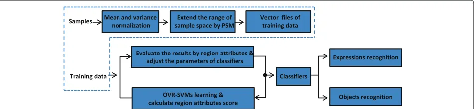
This paper proposes a robust classification framework, which brings together effective normalization measures, visual features, and image attributes to construct a use-ful system. The overview of the proposed framework is shown in Figure 1. There are three main approaches with emphasis on reducing training samples and improving the efficiency of learning machines. First, PSM is used to extend the training data space, which allows us to gen-erate ideal strong classifiers without having to collect a large number of training samples. Second, the features are described by local multi-dimensional SURF descrip-tors [5], which are spatial regions with windows that are good at processing real-time scenes. Moreover, the recog-nition window is scanned across the image at all scales by conventional methods. This paper, however, concentrates on the recognition patches based on SURF interested points. In this way, the framework can become much faster and more efficient. Third, the region attributes of images are adopted to revise incorrect recognition of classifiers relying on visual features, which are repre-sented by feature vectors in a segmented region. There-fore, the discriminative capability can guarantee that the
proposed framework will be more robust. After the PSM approaches, the framework will generate the extended sample space as vector data files. In practice, SVMs can process these vector data files better and faster than the other model classifiers. Therefore, the classifier of our method is based on SVMs.
There are three main ways that the research described in this paper will contribute to the research being carried out in this field. The first is that the efficiency of SVM learn-ing can be improved. Experiments show that the proposed approach is capable of reducing the number of samples effectively, resulting in an obvious reduction in training time. The second benefit is that the recognition accu-racy is comparable to state-of-the-art algorithms. Third, this new system’s versatility is excellent, allowing it to be applied not only to object recognition but also facial expression recognition.
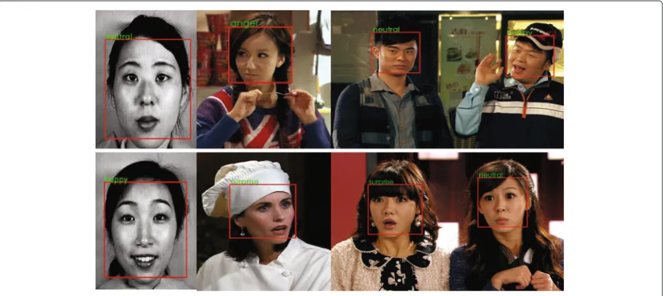
Some examples of expression recognition results are shown in Figure 2. The experimental results show that, despite using a mini-sized database of training samples, our approaches can also construct a robust recognition system, which is comparable to state-of-the-art meth-ods. Moreover, versatility is one of its outstanding traits because, in our experiments, it could succeed in both object recognition and facial expression recognition appli-cations. We believe applying the proposed method to different fields is a good idea because training efficiency and recognition accuracy play very significant roles in machine learning. Also, without a doubt, versatility is equally important.
In the remainder of this paper, we first revisit related works in Section 2. Then, we describe the normalization of samples in Section 3 and the classifying framework in Section 4, respectively. Section 5 describes the experi-ments, and conclusions are drawn in Section 6.
2 Related work
We will first revisit related works on object recognition and facial expression recognition in this section. On one
Figure 2Examples of facial expression recognition results.
hand, facial expression recognition is a typical multi-class multi-classification problem in computer vision. There are many precursors who have focused on FER research, and the latest ones, such as, Liu et al’s STM-ExpLet [6] and Huang et al’s new feature extraction algorithm for FER [7] have pushed the research forward. But many diffi-culties still exist in this research, because the subjects in the images usually have variable facial appearances and they can adopt a wide range of head poses. These problems are difficult to be overcome. Moreover, clas-sifiers usually have to rely on a large-scale dataset for training. Unfortunately, current approaches of FER usu-ally ignore these problems and do not present a robust feature set and a corresponding robust classifying frame-work that allows the expression to be discriminated cleanly under these situations. Reviewing [8] makes it clear that this situation has not been well improved. Looking deeper into the experimental reports of these works [9-13], we also find that the best precision achieved by any of these state-of-the-art methods is no higher than 31.7%, when the method is evaluated by real-world scenarios. Therefore, FER is still an extremely challeng-ing task in computer vision. The first need is a robust feature and the corresponding high-quality training framework.
On the other hand, object recognition is also another hot research topic in computer vision due to its many applications. Great advances have been made in the past decade, especially since the milestone work by Viola and Jones [3]. But we must note that, even with the Viola-Jones method, in order to realize good generalization perfor-mance, more training data are required in the learning
procedure. Although it is quite easy to collect many train-ing samples from the Internet nowadays, collecttrain-ing a large number of samples for training these object detectors [14-16] by search engines is easier said than done. To our knowledge, almost all existing object detectors require large amounts of data for training. Meanwhile, many methods are based on boosting cascade frameworks, and, as we know, almost all existing cascade frameworks are trained based on two conflicted criteria (false-positive-rate and hit-(false-positive-rate) for the detection-error tradeoff. Also known is the fact that training is usually required to achieve a very low false-positive rate per scan window (FPPW) such as 10−6 [17], which means that hundreds of millions or even billions of negative samples should be processed during the training procedure. Therefore, training ideal classifiers is a very time-consuming task. Usually, many researchers have to obtain mirror images of samples for training with the help of third-party software tools.
deal with the samples in order to get mirror images of these samples.
3 PSM for extending sample space
The PSM is derived from the perturbation method, and it can be applied to reducing the size of processing data. For example, it can be used to normalize facial and object data, which is usually adopted as a many-one mapping model. However, in this paper, what we are proposing is a one-many mapping model. Namely, we use it to extend the subspace of samples and the technical details of this one-many mapping model are discussed in this section. In addition, there are also many existing methods based on virtual images, which seem similar to ours, but most of them rely on pixel-level transformation (such as [18,19] etc.). Therefore, after processing with this approach, some features might be damaged easily. Moreover, they require some manual work; and in the training period, the pro-gram has to read a large number of virtual image files again, which leads to time waste. Our approach involves a classification framework that is capable of comput-ing robustly and effectively while avoidcomput-ing the problems mentioned above.
3.1 Training-sample normalization
In order to reduce the noise, the size of the images is unified by m × n pixels, and the original samples are normalized by mean value and variance of pixel transfor-mation. Therefore, the imageIafter normalization can be obtained according to the following equation:
I(x,y)=aI(x,y)−μ
2√2σ +b, (1)
whereσis the standard deviation at the locationsxandy, which can be calculated via
σ=
1
mn
m
x=1
n
y=1
(I(x,y)−μ)2. (2)
(a, b) is used to adjust the value of pixels. In this paper, we used regular samples in experiments; therefore,awas set as 1, andbwas set as 0.μis the mean value of pixels, and it can be computed through image traversal using the following equation:
μ= 1
mn
m
x=1
n
y=1
I(x,y). (3)
3.2 Changing orientational factors
After the calculation of subsection 3.1, we can thus extend the subspace of samples by changing the facial directions of the images. In this paper, we use the method that is pro-posed by Chen et al. [20] on the Procrustes analysis [21] to reconstruct three-dimensional face model and the obtain
three-dimensional data. We indicate it in Algorithm 1. For more details, please refer to Appendix.
Algorithm 1Reconstruct three-dimensional model Require:
Input: two-dimensional shape vector:S2D∈R2;
Output: three-dimensional shape vector:S3D∈R3;
Initialization: setβ0=0,i=0,s0=0; whilei<KorEr> εdo
1. Let
S3D⇐s0+
m
i=1 βisi
2. Alignment: S2D is aligned with the
two-dimensional shape, which is obtained by projecting the frontal three-dimensional shape (si) onto
thex−yplane. 3. Minimize
P(RθS3D+T)−S2D2
4. Reconstruct(S3D)iusing the shape parameterβi.
5. UpdateRθ andT with the fixed shape parameter and
Er ⇐ P(RθS3D+T)−S2D2
6. Let
i⇐i+1
end while
7. Reconstruct three-dimensional shape using the final shape parameters.
8. OutputS3D.
In Algorithm 1, when Er is below a threshold ε
orKlandmarks are processed over, the while loop would be stopped and the three-dimensional data will be out-put. Here,β = (β1,β2,· · ·,βm)T is the shape parameter
andmis the dimensionality of the shape parameter, which is used to adjust three-dimensional shape data.S3Dis a 3×
nmatrix,Pis a 2×3 orthographic projection matrix,Tis a 3×ntranslation matrix consisting ofntranslation vec-torst=[tx,ty,tz]T, andRθis a 3×3 rotation matrix where the yaw angle isθ. In this paper, θis set as±15◦, ±30◦, and±60◦. Thus, through Algorithm 1, we can reconstruct the three-dimensional dataX = (x,y,z)T from the
origi-nal images. Hence, according to the transformation matrix formula,
X=Tz·Ty·Tx·S·Rz·Ry·Rx·X, (4)
shear mapping transformation matrix and the rota-tion matrix respectively, and S represents the scaling matrix.
3.3 Changing illumination attributes
The illuminative change is conducted according to the following equation:
V2(n)=V1(n)+
K
m=1
wm·e(mn), (5)
whereV1is the changing feature,V2is the result after the changes,nis the dimensionality of the feature vector,wis the weight coefficient, andeis the basis of illumination-change-factor vectors.
In this paper, e is obtained through processing the luminance-normalized rendering images by principal component analysis (PCA), wherein, m is the princi-pal component (m = 1,· · ·, 8). The rendering images are gained by the treatment of three-dimensional images obtained in subsection 3.2.
4 Classifying framework
This section will provide the framework used for SVM learning through adopting SURF features. Moreover, we will also employ the region attributes of images to revise the incorrect recognition of classifiers relying on visual features. We will describe them separately in this section.
4.1 Feature description
SURF is a scale- and rotation-invariant interest point detector and descriptor. It is faster than SIFT [22] and more robust against different image transformations. In this paper, we adopt an 8-bin T2 descriptor to describe the local feature, which is inspired by [23]. Unlike [23], however, we further allow different aspect ratios for each patch (the ratio of width and height) because this can make increase the speed of image traversal. We also imported diagonal and anti-diagonal filters because this can improve the description capability of the SURF descriptors.
Given a recognition window, we define rectangular local patches within it, each patch with four spatial cells and allows the patch size ranging from 12×12 to 40×40 pix-els. Each patch is represented by a 32-dimensional SURF descriptor. The descriptor can be computed quickly based on sums of two-dimensional Haar wavelet responses, and we can make an efficient use of integral images [3]. Sup-pose dx as the horizontal gradient image, which can be
obtained using the filter kernel [−1, 0, 1], anddyis the
ver-tical gradient image, which can be obtained using the filter kernel [−1, 0, 1]T; Define dD as the diagonal image and
dADas the anti-diagonal image, both of which can be
com-puted using two-dimensional filter kernels diag(−1, 0, 1) and antidiag(−1, 0, 1). Therefore, 8-bin T2 is able to be defined as v = ((|dx| +dx),(|dx| −dx),(dy+
dy),(dy−dy),(|dD|+dD),(|dD|−dD),(|dAD|+
dAD),(|dAD| −dAD)). Here,dx,dy,dD, anddADcan be
computed individually by filters shown in Figure 3a(1), a(2), b(1), and b(2) respectively in use of integral images, the details about how to compute two-dimensional Haar responses with integral images; please refer to [3].
The recognition template for SURF is 40× 40 with four spatial cells, allowing the patch size ranging from 12×12 to 40×40 pixels. We slide the patch over the recognition template with four pixels forward to ensure enough feature-level difference. We further allow differ-ent aspect ratio for each patch (the ratio of width and height). The local candidate region of the features is divided into four cells. The descriptor is extracted in each cell. Hence, concatenating features in four cells together yields a 32-dimensional feature vector. About feature nor-malization, in practice,L2normalization followed by clip-ping and renormalization (L2Hys) [24] is shown working best.
4.2 Classifier construction
The classifier of our framework is built based on one-versus-rest SVMs (OVR-SVMs). OVR strategy consists of constructing one SVM per class, which is trained to distinguish the samples of one class from the samples of all the remaining classes. Normally, classification of an unknown object is carried out by adopting the max-imum output among all SVMs. The proposed method
is based on OVR-SVMs classifiers and implemented by redeveloping liblinear SDK [25].
For OVR-SVM, the most crucial part is probability estimation. Usually, most researchers estimate posterior probability by mapping the outputs of each SVM into a probability separately. The method was proposed by Platt [26]. It applies an additional sigmoid function:
H(ωj|fj(x))=
1
1+exp(cjfj(x)+dj)
. (6)
fj(x)denotes the output of the SVM trained to separate the
classωjfrom the other classes (total samples areM). Then,
for each sigmoid the parameters,cjanddjare optimized
by minimizing the local negative log-likelihood:
−
N
k=1
{pklog(hk)+(1−pk)log(1−hk)}. (7)
Here are Noutputs of the sigmoid function, wherehkis
the output of the sigmoid function with the probabil-itypkevent. In order to solve this optimization problem,
Platt [26] applied a model-trust minimization algorithm based on the Levenberg-Marquardt algorithm. But in [27], Lin et al. pointed out that there are some problems in this method, meanwhile they proposed another minimization algorithm based on Newton’s method with backtracking line search.
But unfortunately, there is nothing to guarantee that:
M
j=1
H(ωj|fj(x))=1. (8)
For this reason, it is necessary to normalize the proba-bilities as follows:
H(ωj|x)=
H(ωj|fj(x))
M
j=1H(ωj|fj(x))
. (9)
Thus, we use another approach to estimate posterior probability, using OVR-SVMs to exploit the outputs of all SVMs to estimate overall probabilities. In order to achieve this goal, we apply the softmax function, regard-ing it as a generalization of sigmoid function for the multi-SVM case. Hence, in the spirit of the improved Platt’s algorithm [28], this paper applies a parametric form of the softmax function to normalize the probabilities by:
H(ωj|x)=
exp(cjfj(x)+dj)
M
j=1exp(cjfj(x)+dj)
. (10)
The parameterscjanddjare optimized by minimizing
the global negative log-likelihood.
−
N
k=1
log(H(ωk|xk)). (11)
The optimization of parameters cj and dj is done
with the intention of obtaining the lowest error rate on testing dataset. The reason why we use the negative log-likelihood is not only because it can optimize the parame-terscjanddjbut also because it can be used for comparing
the various probability estimates; in other words, it can evaluate the error rate on machine learning and reject some of the unsatisfactory candidate expression regions described by SURF features.
4.3 Region attribute estimation
The detected face/object region is divided intoC=n×m blocks, and the feature vector of each block is computed. These vectors are used to construct a matrixX, which is named as region attributes. Each column data of Xcan be extracted from each block that is normalized by equal-izing the value and variance of the luminance, while the norm is set as 1. The region attribute is estimated using the following score equation.
d=X− ¯X2−
C
i=1 λi
λi+δ2(ϕi(
X− ¯X))2, (12)
where ϕ is the eigenvector of X, λ is the eigenvalue of X, and δ2 denotes the image noise correct divisor. Whenδ2 = 0, it means that the distances of all feature vectors of the current image projecting into subspace are unified; in the other words, the noise is negligible.X is estimated image region attributes, and X¯ is the average feature vector (AFV) of samples. If the value of distance is smaller, the score is higher, namely, the probability of miss-recognition is lower.
Algorithm 2Region attributes for SVM learning.
Require:
1.l−th category AFV:X¯l;
2. Error rate evaluating threshold:e;
3. Positive class samples:S+, samples number: M; 4. Negative class samples:S−, samples number: M;
Initialize:e0=1,d=1,j=0;
for(i=0;i<M;i=i+1)do while(ej>0.5)do
1.j=j+1;
2. Train a set of classifiersH(ωj|fj(x))on samplesS+ andS−via the approaches of subsection 4.2;
3. Using Equation 12 to obtain region attributes score
d;
4.Evaluate the modelH(ωj|fj(x))on the whole training set; ifd>0.2, skip over the step 5 and 6;
5. Update the parameterscjanddjthrough minimizing the global negative log-likelihood on Equation 7; 6. Update the recognition-error tradeoff:ei+1 = ei×
i √
1−d;
7. Empty the setS−;
8.while(ei+1>eiand size|S+| = |S−|) do
Adopt classifier to scan non-target images with sliding window and put false-positive samples intoS−;
end while end while end for
8. Output the probabilities modelH and overall error rate tradeoff parametere.
In order to make the framework more robust, we also adopt two important approaches. 1) If their results are coincident, the region attribute scoredand recognition-error tradeoff parameter e will be updated for the next stage (Algorithm 2, step 3 and step 5); 2) When the results are not coincident, the current image will be put into the negative sample set automatically (Algorithm 2, step 7), so that the classifier can be updated at the next learning iteration stage. Therefore, the proposed framework is an adaptive learning framework that can cover the new data better than the conventional SVM-based methods. At the same time, this framework presents a mutual feedback mechanism for SVMs and the distance metric, which is more robust than a single classifying model. This is very important for avoiding some miss-recognition results that are individually categorized by the classifiers.
5 Experiments
At first, our method was proposed for facial expression recognition. But in practice, we found that it can be successfully applied to not only facial expression recog-nition but also object recogrecog-nition. Therefore, this section will summarize the experimental data for both expres-sion recognition and object recognition. The details of
the implementation, dataset, and evaluation results will be shown here.
5.1 Implementation
We implemented all training and recognition programs in C++ on RHEL (Red Hat Enterprise Linux) 6.5 OS. In expression recognition, the facial detection part used the source code of Open CV, which was based on the Viola and Jones framework [3]. The expressional recognition part was implemented based on the proposed framework. In object recognition, all of the recognition systems were based on the proposed approaches. The experiments were done on the PC (Core i7-2600 3.40 GHz CPU and 8 GB RAM), and the training procedure was fully automatic. For SURF extraction, we adopted the integral image to speedup the computation as described in subsection 4.1. For machine learning, we built the OVR-SVMs through redeveloping liblinear software [25].
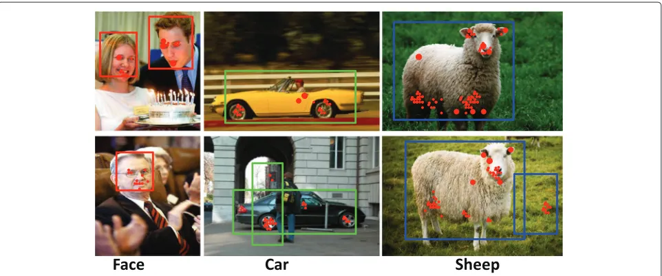
In facial expression recognition, there are neutral-, happy-, anger-, and surprise-expression recognition, and some expression recognition results are shown in Figure 2; In object recognition, the proposed method is designed for classifying faces, cars, and sheep. Some tested exam-ples are shown in Figure 4, where the red patches are SURF interest points. After training, we observed that the SURF interest points mainly lay in the regions of the eyes, mouths, teeth, and noses in face recognition; the regions of the wheels, windshields, and doorknobs in car recogni-tion; and the regions of the ears, noses, and the open space between the legs in sheep recognition.
5.2 Experimental dataset
In the training stage, it is necessary to construct a mini-sized training set for machine learning, which will be applied to fix the parameters of sigmoid and softmax func-tion. In the testing stage, we also need to build the testing set for evaluation. The easiest way to do this is to apply the same dataset to both the training and testing stages in a way of cross-validation. But, as pointed out by Platt [26], using the same data twice can sometimes lead to a dis-astrously biased estimate. Moreover, it cannot be proved that the approach is broadly practical. Therefore, in exper-iments, we used different datasets in the training and testing stages separately. The details of the training set and testing set are shown as follows:
Training database set
Figure 4Examples of object recognition results.
Finally, we obtained 240 initial facial samples for each type of emotion. All of these facial samples were normalized to90×100pixels.
2)Object recognition: a) 213 samples of
JAFFE [30] were used for face training, which were normalized to90×100pixels; b) 600 side view car-training samples from the PASCAL
VOC2007dataset [31] were used for car training, which were normalized to100×250pixels; c) 600 samples were collected using the Google search engine for sheep training, which were normalized to
200×200pixels.
In the training stages, the training data of current pro-cessing category were adopted as positive sample data; the other categories’ data were used for negative data.
Testing database set
1)Expression recognition: In order to evaluate both of the real-life and ideal situations, we used two parts of testing sets. One part was obtained from soap operas, because many public databases were processed by providers in advance or for the other reasons, such as the images cannot represent real-life scenes, because they are not continuous images etc. Hence, we had to use some video clips from comedy dramas, which had a total of ten persons whose facial expressions were similar to the training samples. The images of these actors and actresses are on eight video clips having a length of 120 s. We marked this set as Test Set A. The other testing set was the JAFFE database [30], whose facial samples are totally different from the CK+database. The 213 JAFFE images were mixed randomly, and one image could
be used repeatedly (to ensure that there are enough images for different video making). These images were also made into eight 120-s-long videos, and we marked this set as Test Set B.
2)Object recognition: 80 facial samples collected from the FDDB [32], 80 car-testing samples collected from the PASCAL VOC2005database [31], and 80 samples of sheep collected from NUS-WIDE [33] were mixed and made into three clips of 9-min-long videos. All of the testing videos were normalized to the size of640×480and the frame rate of 60 frames per second (FPS). These videos were used to do evaluation experiments.
5.3 Experimental evaluation 5.3.1 Expression recognition
Training experiments The training database of all meth-ods was mentioned above, but only the proposed method did not adopt any process to obtain plenty of mirror samples. Hence, it reduced a mass of samples and took only 49.8 min to complete the whole process. Besides, the training procedure was fully automatic. The training results are shown in Table 1.
However, in order to enhance the generalization per-formance of comparison methods, we had to deal with the samples by some transformations (mirror reflec-tion and rotate the images by horizontal and vertical angles±15◦, ±30◦, and ±60◦etc.). Finally, we obtained
Table 1 Training efficiency evaluation results
Method Proposed LSH-CORF [9] 3D LUT [20] LBP-TOP [10]
each class 30,960, total 123,840 facial samples for training classifiers. Therefore, they are very time-consuming tasks.
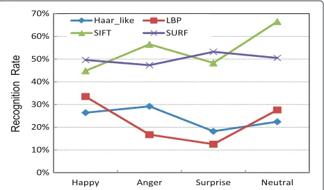
Testing experiments Figure 5 indicates the expression-recognition rate for different feature detectors based on the proposed framework. The aim of this experiment was evaluating the performance of the proposed detec-tor using different methods of feature extraction. Hence, this experiment was done without a PSM model. The results showed that feature detectors using SURF and SIFT obtained more accurate recognition rates, but the average speed of the SIFT detector’s version was only 16.8 FPS. In comparison, the speed of the SURF’s version reached 39.4 FPS. Theoretically, 16.8 FPS is too slow to deal with complex scenes, such as real-time scenes. Our framework adopted an 8-bin T2 descriptor as the descrip-tor. It obtained similarly accurate recognition results com-pared to the accuracy of the original SURF’s version and even the SIFT’s one, but it surpassed the others in regard to feature extraction speed. In fact, in our experiments, 8-bin T2 descriptors had almost the same accuracy as the original SURF; however, the speed of original SURF ver-sion was only about 19 FPS, which was also extremely slow. Therefore, the feature descriptor based on 8-bin T2 SURF is the best choice for our framework.
In Figure 6, the component selection of the proposed method was carried out to investigate how each compo-nent contributes to the recognition rate. As a result, the OVR-SVMs+PSM+SURF model was the most accurate version.
Figure 7 shows the results of the evaluation experi-ments for expressional region attributes. Figure 7a shows the results for Test Set A videos, and Figure 7b shows the results for Test Set B. In the experiments, we found that after introducing the region attributes model, the
Figure 5Expression-recognition rates on different features. Green: recognition rate for OVR-SVMs with SIFT. Purple: recognition rate for OVR-SVMs with SURF. Blue: recognition rate for OVR-SVMs with Haar-like. Red: recognition rate for OVR-SVMs with LBP. Features using SURF and SIFT obtained the more accurate results, but the feature extraction speed of SIFT was low.
Figure 6Expression-recognition rates based on different component selection.Top: recognition rate for proposed method. Middle: proposed method without PSM; i.e., the OVR-SVMs+SURF model. Bottom: OVR-SVMs adopting the image RGB pixel value. OVR-SVMs+PSM+SURF (proposed method) is the most accurate version of our detector.
recognition accuracy of Test Set A improved approxi-mately by 7%. On the other hand, the results of Test Set B were almost unchanged, since the videos in Test Set B consisted of JAFFE images, and these images had been normalized by the supplier [30]. But the videos of Test Set A were used without any normalization. Therefore, this approach is capable of dealing with original images better; i.e., it is good at processing real-life videos.
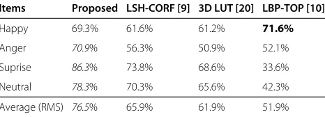
Tables 2 and 3 indicate the recognition accuracies, and they show the performance of the proposed method com-pared to some state-of-the-art methods: 3D LUT [20] and LSH-CORF [9] are the latest methods for facial expres-sions recognition; LBP-TOP [10] is a well-known and classical expression recognition method. All of the com-parison methods were conducted using their released codes, and the data had been tuned to better adapt for our experiments. Note that in this paper, the average pre-cision was evaluated on the root mean square (RMS) of
each expression accuracy, namely, average= Li=1p2i/L (pi denotes the accuracy ofith expression, andL is the
total of expressional categories). Because it can denote the mean level of recognition rate better than mean average precision (mAP) for the event containing different sample numbers in each independent class.
Table 2 shows the recognition rate of evaluation exper-iments for Test Set A. Since the human races and facial expressions of Test Set A’s people were similar to those of the training samples, meanwhile, the region attribute model was effective for Test Set A in which there are videos from real life. Consequently, its accuracy was quite better than the Test Set B’s. The maximum recognition precision of the proposed method was 86.3%, and the worst result was 69.3%.
Figure 7Evaluation results for expressional region attributes.
of facial expressions across different cultures and races, the region attribute model was not effective for facial recognition. The results for this test set were not better than Test Set A’s. But on the whole, the results of both test sets show that the proposed method was the more accurate version of these methods. Note that the proposed method used training samples without any image-mirror process here. Namely, based on the mini-size training set, the proposed method can also obtain a better result; thus, this model allows for generating ideal strong classifiers without the need for large volumes of training samples. Hence, under these experimental conditions, the validity of the proposed methods was proved.
5.3.2 Object recognition
Training experiments As our methods effectively reduce a great number of samples, it took very little time to complete the training process: 2.3 min (face), 10.1 min (car), and 10.6 min (sheep), respectively. The related data are shown in Table 4.
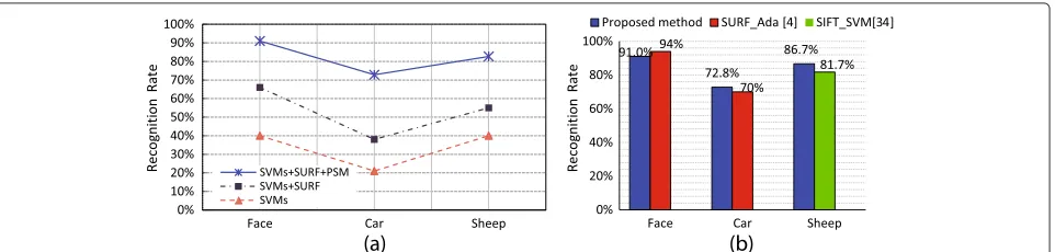
Testing experiments Figure 8 shows the experimen-tal results. In Figure 8a, the component selections of the proposed method were evaluated. The middle one denoted the results of the proposed method without PSM, namely, the OVR-SVM+SURF model. The bottom one indicated the recognition result based on OVR-SVM.
Table 2 Experimental results of expression recognition for Test Set A
Items Proposed LSH-CORF [9] 3D LUT [20] LBP-TOP [10]
Happy 69.3% 61.6% 61.2% 71.6%
Anger 70.9% 56.3% 50.9% 52.1%
Suprise 86.3% 73.8% 68.6% 33.6%
Neutral 78.3% 70.3% 65.6% 42.3%
Average (RMS) 76.5% 65.9% 61.9% 51.9%
The OVR-SVM + PSM + SURF model was also the most accurate version of our object classifier. This also proves the outstanding versatility of the proposed method because it can analyze both human behaviors and object categories.
Figure 8b shows recognition results evaluated by the lat-est detectors. Li et al. [4] claimed they took about 47 min on their PC (Core i7 3.2 GHz CPU and 12 GB RAM) to obtain their ideal facial detectors, which could obtain a precision of 94% (the total of their training samples was 63,000). However, with our approach, using just 213 sam-ples, we were able to achieve similar results. In the other experiment, we gained a little better result, using the same database as Li et al. did for car recognition. On the other hand, for sheep recognition, [34] adopted SIFT features based on SVM to obtain the best accuracy of 81.7% (ver-sus our 86.7%). They did not provide their training time, but there is a reason to believe that the proposed method is better because the amount of their samples is hundreds of times more than ours. We applied similar classifiers; moreover, it was demonstrated that SURF extraction is much faster and more efficient than SIFT in [5].
6 Conclusions
This paper brings together effective normalization mea-sures, visual features, and image attributes to construct a robust classification framework that minimizes the
Table 3 Experimental results of expression recognition for Test Set B
Items Proposed LSH-CORF [9] 3D LUT [20] LBP-TOP [10]
Happy 62.4% 65.3% 57.7% 69.4%
Anger 64.2% 52.0% 48.2% 33.3%
Suprise 79.3% 58.4% 68.4% 42.3%
Neutral 66.5% 71.2% 71.6% 11.7%
Table 4 Total of samples and learning time for object recognition
Method Time cost Sample quantity
Proposed 2.3∼10.6 min
Face: 213
Car: 600
Sheep: 600
SURF_Ada [4] 47 min (face) Face: 63,000 Car: 92,00
SIFT_SVM [34] - - - Sheep: 964,849
amount of training data needed while also improving the training efficiency. It can solve the question how to make classifiers be capable of processing images rapidly and accurately even without having to rely on a large-scale dataset. Hence, it is important to those with closely related research interests.
PSM is an effective approach for alleviating the trou-ble of collecting large amounts of training samples. By carrying out a large number of experiments, we found that SURF is the most suitable feature descriptor for our classifier, and the region attributes of images can revise some incorrectly detected classifiers caused by visual fea-tures. Combining these approaches, a robust classification framework can be constructed, which offers three major advantages. First, it can minimize the amount of train-ing data and improve the traintrain-ing efficiency. Second, the recognition accuracy is comparable to state-of-the-art algorithms. Third, this framework can apply to not only facial expression recognition but also object recognition. The experiments proved the proposed method was valid in regard to training efficiency, recognition accuracy, and versatility.
In future research, considering a possible implementa-tion in a real-life scenario, we are inclined to consider these points: 1) we will try to use region attributes as binary latent variables, which are incorporated into the SVM model for inference, and 2) we will ameliorate meth-ods for the construction of SVMs to improve accuracy and to make our method capable of handling more complex tasks.
7 Appendix
7.1 Additional explanation for Algorithm 1
Procrustes analysis is a statistical tool for analyzing geo-metrical shapes. A shape (or equivalently a figure)PinRP
is represented byllandmarks. Two figuresP:l×pandP: l×p are said to have the same shape, if they are related by a special similarity transformation:
P=αP+IlγT. (13)
where the parameters of the similarity transformation are a rotation matrixΓ:p×p,|| =1, a translation matrixγ: p×l, a positive scaling factorα, andIlis a vector of ones. By using the generalized Procrustes analysis, it is possible to derive a consensus shape for a collection of figures [21], which is then used in registering new shapes into align-ment with the collection by an Affine transformation. In a 3D model, the geometry is defined as a shape vector S3D ∈ R3, which contains thex,y, andzcoordinates ofn vertices. And Equation 13 is adjusted as follows
S=s0+
m
i=1
βisi. (14)
whereβ = (β1,β2,· · ·,βm)T is the shape parameter and
m is the dimension of the shape parameter which was determined to represent the shape of the 3D model. Given the input image indicated asS2D = (x1,y1,· · ·,xn,yn) ∈
R2, the shape parameterβ needs to be determined such that it minimizes the shape residual between the projected 3D facial shape generated by the shape parameter and the input 2D facial shape. The optimal shape and pose parameters(β,Rθ,T)are obtained from
Er= P(RθS3D+T)−S2D2. (15)
whereS3Dis a 3×nmatrix that is reshaped from the 3n×1 model shape vector obtained using Equation 13,Pis a 2×3 orthographic projection matrix,T is a 3×ntranslation matrix consisting ofntranslation vectorst =[tx,ty,tz]T,
andRθis a 3×3 rotation matrix where the yaw angle isθ. The 3D shape creation is indicated as follows:
1. Initialization: setβ0=0andk=1.
2. Alignment:S2Dis aligned with the 2D shape obtained by projecting the frontal 3D shape (si) onto
thex−yplane.
3. UpdateRθandT with the fixed shape parameter by min P(RθS3D+T)−S2D2, and reconstruct (S3D)kusing the shape parameterβk.
4. Verify whetherEr≤ϕork>N; if not, go to step
3 andk=k+1.
5. ReconstructS3Dusing the final shape parameters.
WhenEris below a threshold (e.g. in [21], Gower
sug-gested settingϕ=10−4) or the landmarks are processed over, the reconstruction would be stopped, and the con-sensus shape would be output.
Note:Part content of this Appendix was published in the ACM International Conference on Multimedia 2013.
Competing interests
The authors declare that they have no competing interests.
Acknowledgements
The authors would like to sincerely thank the editors and the anonymous reviewers for their constructive comments and valuable suggestions, which helped to improve this paper.
Author details
1Graduate School of System Informatics, Kobe University, 1-1 Rokkodai, Kobe
657-8501, Hyogo, Japan.2Organization of Advanced Science and Technology,
Kobe University, 1-1 Rokkodai, Kobe 657-8501 Hyogo, Japan.
Received: 27 August 2014 Accepted: 13 February 2015
References
1. Y Freund, R Schapire, A Desicion-theoretic Generalization of On-line Learning and an Application to Boosting. J. Comput. Syst.55(1), 119–139 (1997)
2. LG Valiant, A theory of the learnable. Commun. ACM.27(11), 1134–1142 (1984)
3. P Viola, M Jones, inProc. IEEE Conf. Comput. Vis. Pattern Recognit. (CVPR). Rapid object detection using a boosted cascade of simple features, vol. 1, (2001), pp. 511–5181
4. J Li, Y Zhang, inProc. IEEE Conf. Comput. Vis. Pattern Recognit. (CVPR). Learning SURF cascade for fast and accurate object detection, (2013), pp. 3468–3475
5. H Bay, T Tuytelaars, L Van Gool, inProc. Eur. Conf. Comput. Vis. (ECCV). SURF: speeded up robust features, (2006), pp. 404–417
6. M Liu, S Shan, R Wang, X Chen, inProc. IEEE Conf. Comput. Vis. Pattern Recognit. (CVPR). Learning expressionlets on spatio-temporal manifold for dynamic facial expression recognition, (2014), pp. 1749–1756
7. H-F Huang, S-C Tai, Facial expression recognition using new feature extraction algorithm. Electron. Lett. Comput. Vision Image Anal.11(1), 41–54 (2012)
8. J. J. K. S. RolandGoecke Abhinav Dhall, T Gedeon, inProc. ACM The Int. Conf. on Multimodal Interaction (ICMI). Emotion recognition in the wild challenge 2014, (2014)
9. O Rudovic, V Pavlovic, M Pantic, inProc. IEEE Conf. Comput. Vis. Pattern Recognit. (CVPR). Multi-output Laplacian dynamic ordinal regression for facial expression recognition and intensity estimation, (2012), pp. 2634–2641
10. G Zhao, M Pietikainen, Dynamic texture recognition using local binary patterns with an application to facial expressions. IEEE Trans. PAMI.29(6), 915–928 (2007)
11. L Wang, Y Qiao, X Tang, inProc. IEEE Conf. Comput. Vis. Pattern Recognit. (CVPR). Motionlets: mid-level 3D parts for human motion recognition, (2013), pp. 2674–2681
12. P Scovanner, S Ali, M Shah, inProc. ACM Multimedia Conf. (MM). A 3-dimensional sift descriptor and its application to action recognition, (2007), pp. 357–360
13. A Klaser, M Marszalek, C Schmid, inProc. British Machine Vis. Conf. (BMVC). A spatio-temporal descriptor based on 3D-gradients, (2008), pp. 275–110 14. S Maji, AC Berg, inProc. IEEE Int. Conf. Comput. Vis. (ICCV). Max-margin
additive classifiers for detection, (2009), pp. 40–47
15. Q Zhu, M-C Yeh, K-T Cheng, S Avidan, inProc. IEEE Conf. Comput. Vis. Pattern Recognit. (CVPR). Fast human detection using a cascade of histograms of oriented gradients, vol. 2, (2006), pp. 1491–1498 16. L Bourdev, J Brandt, inProc. IEEE Conf. Comput. Vis. Pattern Recognit. (CVPR).
Robust object detection via soft cascade, vol. 2, (2005), pp. 236–243 17. P Viola, MJ Jones, Robust real-time face detection. Int. J. Comput. Vision.
57(2), 137–154 (2004)
18. W-S Chu, C-R Huang, C-S Chen, Gender classification from unaligned facial images using support subspaces. Inf. Sci.221, 98–109 (2013) 19. D Decoste, B Schölkopf, Training invariant support vector machines.
Machine Learning.46(1-3), 161–190 (2002)
20. J Chen, Y Ariki, T Takiguchi, inProc. ACM Multimedia Conf. (MM). Robust facial expressions recognition using 3D average face and ameliorated adaboost, (2013), pp. 661–664
21. JC Gower, Generalized procrustes analysis. Psychometrika.40(1), 33–51 (1975)
22. DG Lowe, inProc. IEEE Int. Conf. Comput. Vis. (ICCV). Object recognition from local scale-invariant features, vol. 2, (1999), pp. 1150–1157 23. J Li, T Wang, Y Zhang, inProc. IEEE Int. Conf. Comput. Vis. (ICCV) Workshops.
Face detection using SURF cascade, (2011), pp. 2183–2190
24. N Dalal, B Triggs, inProc. IEEE Conf. Comput. Vis. Pattern Recognit. (CVPR). Histograms of oriented gradients for human detection, vol. 1, (2005), pp. 886–8931
25. R-E Fan, K-W Chang, C-J Hsieh, X-R Wang, C-J Lin, LIBLINEAR: a library for large linear classification. J. Machine Learning Res.9, 1871–1874 (2008) 26. J Platt, inProc. Advances in Large Margin Classifiers. Probabilities for SV
machines, (2000), pp. 61–74
27. H-T Lin, C-J Lin, RC Weng, A note on Platt’s probabilistic outputs for support vector machines. Machine learning.68(3), 267–276 (2007) 28. Z Sun, N Ampornpunt, M Varma, S. v. n. Vishwanathan, inProc. Adv. Neural
Inf. Process. Syst. (NIPS). Multiple kernel learning and the SMO algorithm, (2010), pp. 2361–2369
29. P Lucey, JF Cohn, T Kanade, J Saragih, Z Ambadar, I Matthews, inProc. IEEE Conf. Comput. Vis. Pattern Recognit. (CVPR) Workshops. The extended Cohn-Kanade dataset (CK+): a complete dataset for action unit and emotion-specified expression, (2010), pp. 94–101
30. M Lyons, J Gyoba, S Akamatsu, Automatic Classification of Single Facial Images. EEE Trans. PAMI.21(12), 1357–1362 (1999)
31. M Everingham, L Van Gool, CKI Williams, J Winn, A Zisserman, The pascal visual object classes (VOC) challenge. Int. J. Comput. Vision.88(2), 303–338 (2010)
32. V Jain, EG Learned-Miller, FDDB: a benchmark for face detection in unconstrained settings. UMass Amherst Technical Report (2010) 33. T-S Chua, J Tang, R Hong, H Li, Z Luo, Y-T Zheng, inProc. ACM Int. Conf.
Image and Video Retrieval (CVIR). NUS-WIDE: a Real-World Web Image Database from National University of Singapore, (2009)
![Figure 3 Haar-type filter used for computing SURF descriptor. [a(1)] dx, [a(2)] dy, [b(1)] dD, and [b(2)] dAD.](https://thumb-us.123doks.com/thumbv2/123dok_us/911382.1588935/5.595.62.541.630.715/figure-haar-type-filter-used-computing-surf-descriptor.webp)