Volume 17, Number 5 (2019), 879-891
URL:https://doi.org/10.28924/2291-8639 DOI:10.28924/2291-8639-17-2019-879
COMPUTING STRUCTURED SINGULAR VALUES FOR STURM-LIOUVILLE PROBLEMS
MUTTI-UR REHMAN1,∗, GHULAM ABBAS1 AND ARSHAD MEHMOOD2
1Department of Mathematics, Sukkur IBA University, Sukkur-Sindh 65200 Pakistan
2Department of Mathematics, The University of Lahore, Gujrat campus, Gujrat-Punjab 50700 Pakistan
∗Corresponding author: [email protected]
Abstract. In this article we present numerical computation of pseudo-spectra and the bounds of Structured Singular Values (SSV) for a family of matrices obtained while considering matrix representation of Sturm-Liouville (S-L) problems with eigenparameter-dependent boundary conditions. The low rank ODE’s based technique is used for the approximation of the bounds of SSV. The lower bounds of SSV discuss the instability analysis of linear system in system theory. The numerical experimentation show the comparison of bounds of SSV computed by low rank ODE’S technique with the well-known MATLAB routine mussv available in MATLAB Control Toolbox.
1. Introduction
The spectrum of a matrix Sturm-Liouville (S-L) problem was characterized by F.V.Atkinson in terms of
the spectrum of a class of unitary matrices in his famous book titled Discrete and continuous boundary value
problems. The Atkinson’s team had developed a prototype FORTRAN code in order to numerically compute
the spectrum of S-L problems [1]. The spectrum of a regular, self-adjoint S-L problem is not bounded and
therefore as a result is infinite. The spectrum of a regular, self-adjoint S-L problem is bounded and finite
when the coefficients of S-L problem satisfies the external imposed conditions. For a positive integer n,
exactlyneigenvalues are computed for a class of S-L problems [2]. The finite spectrum to S-L problem while
Received 2019-06-12; accepted 2019-07-17; published 2019-09-02.
2010Mathematics Subject Classification. 15A18, 15A03, 80M50.
Key words and phrases. eigen values; singular values; singular vectors; low rank ODE’s.
c
2019 Authors retain the copyrights
of their papers, and all open access articles are distributed under the terms of the Creative Commons Attribution License.
considering the transmission conditions are studied in [3] which shows the equivalent matrix representation.
The matrix representation of S-L problems for eigen parameter dependent boundary conditions are studied
in [4–6].
A S-L problem is one of the form
−(p y0)0+q y=λW y
on an open interval I = (a, b) with −∞ < a < b < ∞ having the eigen parameter dependent boundary
conditions of the form
AηΘ(a) +BηΘ(b) = 0, Θ = (y py0)t
with
Aη=
ηα0
1−α1 −ηα02+α2
0 0
, Bη=
0 0
ηβ10 +β1 −ηβ20 −β2
,
whereαi, α0i, βi, βi0∈R, ∀i= 1 : 2, such that
ξ1=α01α2−α1α02= 0, ξ6 2=β10β2−β1β026= 0.
The parameter η is the spectral parameter while the coefficients satisfying the minimal conditions r = 1
p, q, w∈L(I,C) whereL(I,C) is the complex valued function which are Lebesgue integrable on the interval I.
The S-L problem as considered above is said to be of Atkinson type if forn >1 there exists
a=a0< b0<· · ·< an< bn=b
withr= 1p = 0 on [ak, bk],Wk = Rbk
ak W dW 6= 0, ∀k= 1 :n andq=W = 0 on [bk−1, ak], rk =
Rbk
akr dr6=
0, ∀k= 1 :n.
The S-L problem with the eigen parameter dependent boundary conditions is equivalent to matrix eigenvalue
problem of the form
(P+Q)U =ηW U
whereU = [v0, u0, u1, ..., un, vn+1] is an eigenvector. This finally lead us to the following eigenvalue problem
where we aim to approximate eigenvalues ηi, singular values σi and structured singular values µi of the
matrix (P+Q)W−1with
(P+Q)U =ηW U,
in turns this implies that
(P+Q)W−1−ηIU = 0.
The Singular Value Decomposition (SVD) is one of the important tool in the modern days numerical analysis
and specially in numerical linear algebra. The applications of SVD and it’s basic theory are studied in [7].
SVD tool splits up matrix A into further three matricesU,Σ and Vt. The matrix Σ is the one look like
as a diagonal matrix and having the non-negative quantitiesσi along it’s main diagonal. The quantitiesσi
are known as the singular values ofA. The singular values are the positive square roots of the spectrum of
matrixAtA rather thanA. The columns vectors ofU are known as the left singular vectors ofAwhile the
orthonormal eigen vectors ofAAt. On the other hand, the column vectors of the orthogonal matrixV acts
as the right singular vectors ofAand orthonormal eigen vectors forAtA. Both singular values and singular
vectors are relatively insensitive to the perturbations across the elements of the matrix under consideration.
These quantities are also insensitive to finite precision error [8]. The singular values are well-conditioned
with respect to an accuracy [9].
Golub-kahan-Reinsch singular value decomposition algorithm [10] is the standard numerical algorithm used
for the approximation of the singular values of a matrix. Hestenes algorithm [11] and Kogbetliantz
algo-rithm [12] acts as the parallel algorithms for the computation of the singular values σi. The algorithm by
Golub-kahan-Reinsch is computationally very efficient on the sequential machine but however it’s not much
attractive on the parallel processor [13].
The Structured Singular Values (SSV) is the generalization of the singular values of a square, rectangular
matrixA ∈ Km,n with K=R,C. SSV was first introduced by J.C.Doyle [14]. The SSV tool widely used
in control, system theory to investigate both stability and instability of feedback systems. For applications
we refer [15]. Unfortunately, the computation of an exact value of SSV is not possible and appear as an
NP-hard problem [17] which allows to develop numerical methods in order to approximate bounds of SSV.
The lower bounds of SSV are approximated by using power method [16] while [18] is used to approximate
it’s upper bounds. The lower bounds of SSV provide sufficient information about the instability of closed
loop system while upper bounds is used to study the stability of feedback system in linear control theory.
1.1. Preliminaries.
Definition 1.1. The spectrum of a square a complex valued matrix M ∈Cn,n is defined as
Λ(M) ={λ∈C: |(λI−M)|= 0}.
Definition 1.2. The pseudospectrum of a complex matrix M ∈ Cn,n with a small positive real parameter
>0 is defined as
Λ(M) ={λ∈C: |(λI−M)−1| ≥ 1
}.
Definition 1.3. For a small positive parameter ≥0. A number λ belongs to epsilon-pseudo-spectrum of
an operatorA, denoted byΛ(A)and satisfies the following equivalent conditions
(ii) ∃u∈Cn,n having kuk= 1 such that kAu−λuk ≤;
(iii)λ∈ρ(A)andk(λI−A)−1k ≥ 1
orλ∈Λ(A)where ρ(A)denotes the spectral radius of the matrix A.
Definition 1.4. The pseudospectrum of a complex matrix M ∈ Cn,n with a small positive real parameter
>0 is defined as
Λ(M) ={λ∈C: |(λI−M)−1| ≥
1 }.
Definition 1.5. Unstructured uncertaintyBor stuctured uncertaintyBis stable transfer matrix or structured
stable transfer matrix having the form.
B={diag(δiIi; ∆j) :δi∈C,∆j ∈Cmj,mj,∀i= 1 :S, j= 1 :F}.
Definition 1.6. For a given n-dimensional square matrixM ∈Cn,n and underlying perturbation setB, the
µ-value is defined as
µB(M) = 1
min{k∆k2: ∆∈B, det(I−M∆) = 0}
.
unless no such∆ cause(I−M∆) to be singular for whichµB(M) = 0.
1.2. Reformulation of µ-values. In this section we reformulate theµ-values on the basis of structured
spectral value sets. The key idea for the reformulation of the structured singular values is to shift the largest
eigenvalue of the matrix valued function I−M∆(t) such that forλmax = 1 the new eigenvalue η = 0 as
η= 1−λmaxand it achieve the maximum value to be one whenλmax= 0.On the basis of this mathematical
construction, the reformulation of structured singular values is given as below.
Definition 1.7. For a given M ∈ Cn,n and perturbation level > 0, the structured spectral value set is
denoted byΛB
(M)and is defined as
ΛB
(M) ={λ∈Λ(M∆),∆∈B,k∆k2≤1},
whereΛ(M∆)denotes the spectrum of the matrix valued function(M∆), and is simply a disk centered at
origin 0.
Definition 1.8. The structured epsilon spectral value set for a given M ∈Cn,n and≥0, is defined as
ΣB
(M) ={η: 1−λ:λ∈ΛB(M)}.
Definition 1.9. For a given M ∈Cn,n and an underlying perturbation setBthe µ-value is defined as
µB(M) = 1
2. Pseudo-Spectrum
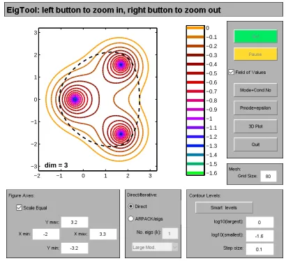
In this section we present the pseudospectra for matrices under consideration to whom the goal is to
approximate structured singular values. For this purpose we make use of the software package EigTool [19].
EigTool is routinely used for plotting unstructured pseudospectra of the matrices under consideration. In
Figures 1-4, we show the computation of the pseudospectra of a different matrices as taken in examples
1-4. We also show the absolute values and the real part of the eigenvalues computed for each matrix. The
spectrum of the eigenvalues in 3-dimensional space is also shown by making use of Eigtool.
LetAbe an n-dimensional matrix and let Λ(A) denotes the set of all the eigenvalues of the matrixA. Let
kAkdenotes the matrix-norm of the matrixAinduced by an inner product spaceh·,·i. The computation of
the pseudo-spectra of an operator is very straightforward but at the same its very costly too. The boundaries
associated with the pseudo-spectrum are nothing but just the level curves of the resolvent corresponding to
operator A, that is, k(λI−A)−1k. The computations of the level curves involves the computation of the
numerical values ofλat the grid point in the complex planes and then to compute the desired contour plots.
For the computation of the-pseudo-spectrum, the computation of an admissible perturbationE such that
kEk=for the perturbed matrixA+E. For the computation of the-pseudo-spectrum the determination
of the setsL andU is essential such thatL≤Λ≤U.
Here, L(A) ={λ∈ρ(A) :b(λ) ≥ 1
} ∪Λ(A) acts as a lower bound of the -pseudo-spectrum with ≥0. For an upper bounds of the pseudo-spectrum,U(A) ={λ∈ρ(A) :B(λ)≥ k(λI−A)−1k}for allλ∈ρ(A).
For a complete detail we refer [20] and the reference therein.
dim = 3
−2 −1 0 1 2 3 −3
−2 −1 0 1 2 3
−1.6 −1.5 −1.4 −1.3 −1.2 −1.1 −1 −0.9 −0.8 −0.7 −0.6 −0.5 −0.4 −0.3 −0.2 −0.1 0
(a)Pseudospectrum of 3-dim real valued matrix
Figure 1. Matlab interface for computing pseudospectrum. The graphical representation
dim = 4
−2 0 2 4 6 8
−4 −3 −2 −1 0 1 2 3 4
−1.4 −1.3 −1.2 −1.1 −1 −0.9 −0.8 −0.7 −0.6 −0.5 −0.4 −0.3 −0.2 −0.1 0 0.1 0.2 0.3
(a)Pseudospectrum of 4-dim real valued matrix
Figure 2. Matlab interface for computing pseudospectrum. The graphical representation
show the pseudospectrum of the 4-dimensional real valued matrix (Example 2)
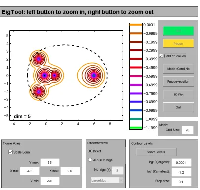
dim = 5
−4 −2 0 2 4 6 8 −5
−4 −3 −2 −1 0 1 2 3 4 5
−1.1999 −1.0999 −0.9999 −0.8999 −0.7999 −0.6999 −0.5999 −0.4999 −0.3999 −0.2999 −0.1999 −0.0999 0.0001
(a)Pseudospectrum of 5-dim real valued matrix
Figure 3. Matlab interface for computing pseudospectrum. The graphical representation
dim = 6
−5 0 5 10 15
−6 −4 −2 0 2 4 6
−1.2 −1.1 −1 −0.9 −0.8 −0.7 −0.6 −0.5 −0.4 −0.3 −0.2 −0.1 0 0.1 0.2 0.3 0.4 0.5
(a)Pseudospectrum of 6-dim real valued matrix
Figure 4. Matlab interface for computing pseudospectrum. The graphical representation
show the pseudospectrum of the 6-dimensional real valued matrix (Example 4)
3. Proposed Methodology
In order to solve the maximization problem discussed in Definition 3.3, we make use of numerical method
based upon low-rank ordinary differential equations technique. The numerical method is mainly composed of
two-level algorithm, that is, inner-algorithm and outer-algorithm. In the inner-algorithm the main objective
is to first construct then solve a gradient system of ordinary differential equations. On the other hand in
the Outer-algorithm we vary the perturbation level > 0 by means of fast Newton iteration. The
outer-algorithm computes an exact derivative of an extremizer say ∆() for ∆∈B and >0. A complete detail
of numerical method under consideration is given in [15].
Next, we discuss the computation of an extremizer. For this purpose, we first approximate the derivative
of an eigenvalue matrix Λ(p) of a smooth matrix family say A(p) for some fixed parameterp.
3.1. Approximation of an Extremizers. A matrix valued function ∆ ∈ B having the largest singular
value bounded above by 1 and the matrix valued function (I−M∆) having a smallest eigenvalue which
minimizes the modulus of structured spectral value setPB
(M) is known as an extremizer. The following theorem computes extremizer for a chosen smallest complex number belonging to the setPB
(M). Theorem 5.1. For a perturbation ∆∈Bhaving the block diagonal structure
withk∆k2= 1, acts as a local extremizer of structured spectral value set. For a simple smallest eigenvalue
λ = |λ|eιθ, θ ∈ R of matrix valued function (I−M∆) having right and left evectors xand y scaled as
S=eιθy∗xand letz=M∗y. The non-degeneracy conditions
z∗
kxk6= 0, ∀= 1 :S
0
Re(zk∗xk)6= 0, ∀= 1 :S
0
+ 1 :S
and ||zs+h||.||xs+h|| 6= 0, ∀h= 1 :F,
holds. Then magnitude of each complex scalarδi∀i= 1 :sappears to be exactly equal to 1 while each full
block possesses a unit 2-norm.
3.2. Gradiant System of ODE’s. The gradient system of odes for an admissible perturbation ∆∈B to
approximate a local extremizer of smallest eigenvalueλ=|λ|iθ, is obtained as,
˙
δi=νi(x∗izi−Re(x∗iziδi)δi);¯ i= 1 :s0 ˙
δl=sign(Re(z∗lxl)Ψ(−1,1)(δl); l=s 0
+ 1 :s ˙
∆j =νj(zs+jx∗s+j−Reh∆j;zs+jx∗s+ji); j= 1 :F,
whereδi∈C,∀i= 1 :s 0
, δl∈Rforl=s 0
+ 1 and Ψ(−1,1), the characteristic function. For more discussion
in the construction of gradient system of odes in above equations, we refer to [15].
3.3. Outer-Algorithm. In outer-algorithm the main aim is to vary >0, the perturbation level by means
of fast Newton’s itaration. In turn 1
will provide us the approximation of lower bound ofµ-value. We make use of fast newton’s iteration in order to solve a problem
|λ()|= 1, (3.1)
In Eq. (5.1), >0.In order to solve Eq. (5.1), we need to compute
d
d(|λ()|),
the derivative.
The following theorem (5.2) help us to compute d
d(|λ()|), when |λ()| is simple and ∆(0), λ(0) are assumed to remains smooth in the neighboring region of perturbation level >0
Theorem 5.2Consider matrix valued function ∆∈B. Letxand y as a function of perturbation level
> 0 acts as right and left eigenvectors of matrix valued function (M∆). Consider the scaling of these
vector accordingly of theorem (5.2). Let z=M∗y and assume that non-degenracy conclusions as discussed
in theorem (5.2) yields then, d
d(|λ()|) = 1
|y(∗)x()|
s X
i=1
|zi()∗xi()|
+ F X
j=1
3.4. Choice of suitable initial value matrix and initial perturbation level. For a suitable choice of
the initial value matrix ∆0and an initial perturbation level0, we refer to [15].
4. Numerical Experimentation
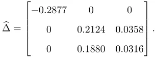
Example 1.
Consider a three dimensional real valued matrixM = (P+Q)W−1 taken from [21].
M =
−1 −2 0
1 2 2
0 −1 2
.
We take the underlying perturbation as
ΘB={diag(δ1I1,∆1) :δ1∈R, ∆1∈C2,2}.
The well-known MATLAB routine mussv approximates the bounds of SSV as follows along with the required
perturbation∆ asb
b ∆ =
−0.2877 0 0
0 0.2124 0.0358
0 0.1880 0.0316
.
We compute the matrix 2-norm of∆, that is,b k∆bk2= 0.2877.The mussv routine computes an upper bound
µupperP D = 3.4762 meanwhile a same lower bound is computedµlower
P D = 3.4762. Algorithm [15] computes the
lower bounds of SSV as follows while the admissible perturbation∗∆∗ is obtained as
∆∗=
−1 0 0
0 0.7384 0.1243
0 0.6537 0.1100
.
The perturbation level is computed as∗ = 2 and an admissible perturbation possesses a unit 2.norm, that
is,k∆∗k2= 1.The lower bound of SSV is obtained asµlowerN ew = 3.4762.
Figure. 9 shows the numerical approximations of both lower and an upper bound of SSV. The graphical
interpretation shows that in various cases the obtained results for the lower and upper bounds of SSV via
Low rank ODE’s and MATLAB routine mussv are similar. In some cases it’s clear that obtained results via
0 0.5 1 1.5 2 2.5 3 3.5 4 2.2
2.4 2.6 2.8 3 3.2 3.4 3.6 3.8
Frequency(rad/sec)
Upper/Lower bounds by mussv
Upper bounds by mussv Lower bounds by mussv Lower bounds by NAlgo
Figure 5. Comparison of the bounds of SSV approximated by MATLAB function mussv
and NAlgo for a 3-dim real matrix valued function at frequenciesw= 1 : 5.
Example 2. Consider a four dimensional real valued matrixM = (P+Q)W−1 taken from [21].
M =
−1 −6 0 0
1 6 1.3333 0
0 4 2 1.5
0 0 0.6667 1
.
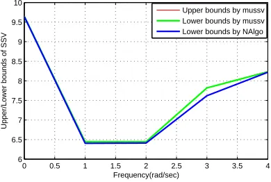
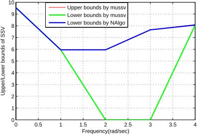
Figure. 10 shows the numerical approximations of both lower and an upper bound of SSV. The graphical
interpretation shows that in various cases the obtained results for the lower and upper bounds of SSV via
Low rank ODE’s and MATLAB routine mussv are similar. In some cases it’s clear that obtained results via
mussv for the lower bounds of SSV dominates than those obtained by Low rank ODE’s technique.
0 0.5 1 1.5 2 2.5 3 3.5 4
6 6.5 7 7.5 8 8.5 9 9.5 10
Frequency(rad/sec)
Upper/Lower bounds of SSV
Upper bounds by mussv Lower bounds by mussv Lower bounds by NAlgo
Figure 6. Comparison of the bounds of SSV approximated by MATLAB function mussv
Example 3.
Consider a five dimensional real valued matrixM = (P+Q)W−1 taken from [21].
M =
−1 −6 0 0 0
1 6 1.3333 0 0
0 4 0 −1.5 0
0 0 2.6667 −1 0.5
0 0 0 0.5 1
.
Figure. 11 shows the numerical approximations of both lower and an upper bound of SSV. The graphical
interpretation shows that in various cases the obtained results for the lower and upper bounds of SSV via
Low rank ODE’s and MATLAB routine mussv are similar. In some cases it’s clear that obtained results via
mussv for the lower bounds of SSV dominates than those obtained by Low rank ODE’s technique.
0 0.5 1 1.5 2 2.5 3 3.5 4
0 1 2 3 4 5 6 7 8 9 10 Frequency(rad/sec)
Upper/Lower bounds of SSV
Upper bounds by mussv Lower bounds by mussv Lower bounds by NAlgo
Figure 7. Comparison of the bounds of SSV approximated by MATLAB function mussv
and NAlgo for a 5-dim real matrix valued function at frequenciesw= 1 : 5.
Example 4.
Consider a six dimensional real valued matrixM = (P+Q)W−1taken from [21].
M =
−1 −6 0 0 0 0
1 6 1.3333 0 0 0
0 4 0 −1.5 0 0
0 −6 −0.6667 2.5 0 0
0 0 0 −2 12 0.5
0 0 0 0 2 1
.
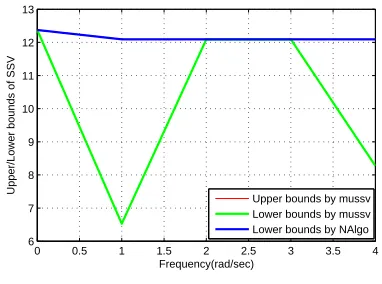
Figure. 12 shows the numerical approximations of both lower and an upper bound of SSV. The graphical
Low rank ODE’s and MATLAB routine mussv are similar. In some cases it’s clear that obtained results via
mussv for the lower bounds of SSV dominates than those obtained by Low rank ODE’s technique.
0 0.5 1 1.5 2 2.5 3 3.5 4
6 7 8 9 10 11 12 13
Frequency(rad/sec)
Upper/Lower bounds of SSV
Upper bounds by mussv Lower bounds by mussv Lower bounds by NAlgo
Figure 8. Comparison of the bounds of SSV approximated by MATLAB function mussv
and NAlgo for a 6-dim real matrix valued function at frequenciesw= 1 : 5.
5. Conclusion.
In this article we have presented numerical computation of pseudo-spectra and the bounds of
struc-tured singular values (SSV) for a family of matrices obtained while considering the matrix representation of
Sturm-Liouville (S-L) problems with eigenparameter-dependent boundary conditions. The numerical
exper-imentation shows that:
•In some cases the lower bounds of SSV obtained by Low rank ODE’s based technique are sharper than the
one approximated by MATLAB routine mussv.
•The MATLAB routine mussv is very fast compare to Low rank ODE’s based technique.
• The MATLAB routine mussv additionally approximate an upper bounds of SSV which is not possible
while making use of Low rank ODE’s based technique.
References
[1] Atkinson, FV and Krall, AM and Leaf, GK and Zettl, A. On the numerical computation of eigenvalues of matrix Sturm-Liouville problems with matrix coefficients. Argonne National Laboratory Reports, Darien, 1987.
[2] Kong, Q and Wu, H and Zettl, A. Sturm–Liouville problems with finite spectrum. J. Math. Anal. Appl., 263 (2001) 748–762.
[3] Ao, Ji-jun and Sun, Jiong and Zhang, Mao-zhu. The finite spectrum of Sturm–Liouville problems with transmission conditions. Appl. Math. Comput., 218 (2001), 1166–1173.
[5] Ao, Ji-jun and Sun, Jiong and Zhang, Mao-zhu. Matrix representations of Sturm–Liouville problems with transmission conditions. Computers Math. Appl., 63 (2012), 1335–1348.
[6] Ao, Ji-jun and Sun, Jiong and Zhang, Mao-zhu. The finite spectrum of Sturm–Liouville problems with transmission conditions and eigenparameter-dependent boundary conditions. Results Math., 63 (2013), 1057–1070.
[7] Vandewalle, Joos and De Moor, Bart. A variety of applications of singular value decomposition in identification and signal processing. SVD Signal Proc. Algorithms Appl. Architect Amsterdam, 1988, 43–91.
[8] Wilkinson, James Hardy. The algebraic eigenvalue problem. Oxford Clarendon, vol. 662, 1965.
[9] Klema, Virginia and Laub, Alan. The singular value decomposition: Its computation and some applications. IEEE Trans. Automatic Control, 25 (1980), 164–176.
[10] Golub, Gene and Kahan, William. Calculating the singular values and pseudo-inverse of a matrix. J. Soc. Ind. Appl. Math., Ser. B, Numer. Anal., 2 (1965), 205–224.
[11] Hestenes, Magnus R. Inversion of matrices by biorthogonalization and related results. J. Soc. Ind. Appl. Math., 6 (1958), 51–90.
[12] Kogbetliantz, EG. Solution of linear equations by diagonalization of coefficients matrix. Q. Appl. Math., 13 (1955), 123–132.
[13] Luk, Franklin T. Computing the singular value decomposition on the ILLIAC IV. Cornell University, year. 1980. [14] Doyle, John. Analysis of feedback systems with structured uncertainties. IEE Proc., Part D , 129 (1982), 242–250. [15] Guglielmi, Nicola and Rehman, Mutti-Ur and Kressner, Daniel. A novel iterative method to approximate structured
singular values. SIAM J. Matrix Anal. Appl., 38 (2017), 361–386.
[16] Packard, Andy and Fan, Michael KH and Doyle, John. A power method for the structured singular value. Proc. 27th IEEE Conf. Decision Control, 1988, 2132–2137.
[17] Braatz, Richard P and Young, Peter M and Doyle, John C and Morari, Manfred. Computational complexity ofµcalculation. IEEE Trans. Automatic Control 39 (1994), 1000-1002.
[18] Fan, Michael KH and Tits, Andr´e L and Doyle, John C. Robustness in the presence of mixed parametric uncertainty and unmodeled dynamics. IEEE Trans. Automatic Control 39 (1994), 25-38.
[19] Wright, Thomas G and Trefethen, LN. Eigtool. Software available at http://www.comlab.ox.ac.uk/pseudospectra/eigtool, 2002.
[20] Reddy, Satish C and Schmid, Peter J and Henningson, Dan S. Pseudospectra of the Orr–Sommerfeld operator. SIAM J. Appl. Math., 53 (1993), 15–47.