University of Pennsylvania
ScholarlyCommons
Publicly Accessible Penn Dissertations
2018
Essays On Banking And Asset Pricing
Tetiana Davydiuk
University of Pennsylvania, tetianad@andrew.cmu.edu
Follow this and additional works at:
https://repository.upenn.edu/edissertations
Part of the
Finance and Financial Management Commons
This paper is posted at ScholarlyCommons.https://repository.upenn.edu/edissertations/2985 For more information, please contactrepository@pobox.upenn.edu.
Recommended Citation
Essays On Banking And Asset Pricing
Abstract
This dissertation consists of two chapters. In the first chapter, I study both theoretical and quantitative implications of the counter-cyclical capital buffers introduced with the Basel Accord III. The proposed adjustment effectively translates into capital charges that vary over time. To this end, I develop a tractable general equilibrium model and use it to solve for optimal state-dependent capital requirements. An optimal policy trades off reduced inefficient lending with reduced liquidity provision. Quantitatively, I find that the optimal Ramsey policy requires pro-cyclical capital ratios that mostly vary between 4% and 6% and depend on the output and bank credit growth, as well as the liquidity premium. Specifically, a one standard deviation increase in GDP (bank credit) translates into 0.6% (0.1%) increase in the capital charges, while a one standard deviation increase in liquidity premium leads to a 0.2% drop. The welfare gain of implementing this Ramsey policy is relatively large.
In the second chapter, I, jointly with Scott Richard, Ivan Shaliastovich and Amir Yaron, investigate the channels of asset price variation when a representative agent owns the entire corporate sector. Utilizing novel market data on corporate bonds we measure the aggregate market value of U.S. corporate assets and their payouts to investors. Total asset payouts are very volatile, turn negative when corporations raise capital, and in contrast to procyclical cash payouts are acyclical. This challenges the notion of risk and return since the risk premium on corporate assets is comparable to the standard equity premium. To reconcile this evidence, we show that aggregate net issuances, which are acyclical and highly volatile, mask a strong exposure of total payouts’ cash components to low-frequency growth risks. We develop an asset-pricing framework to quantitatively assess this economic channel.
Degree Type
Dissertation
Degree Name
Doctor of Philosophy (PhD)
Graduate Group
Finance
First Advisor
Joao Gomes
Second Advisor
Amir Yaron
Subject Categories
ESSAYS ON BANKING AND ASSET-PRICING
Tetiana Davydiuk
A DISSERTATION
in
Finance
For the Graduate Group in Managerial Science and Applied Economics
Presented to the Faculties of the University of Pennsylvania
in
Partial Fulfillment of the Requirements for the
Degree of Doctor of Philosophy
2018
Co-Supervisor of Dissertation
Joao Gomes, Howard Butcher III Professor of Finance
Co-Supervisor of Dissertation
Amir Yaron, Robert Morris Professor of Banking & Finance
Graduate Group Chairperson
Catherine M.Schrand, Celia Z. Moh Professor Professor of Accounting
Dissertation Committee
Itay Goldstein, Joel S. Ehrenkranz Family Professor of Finance
ESSAYS ON BANKING AND ASSET-PRICING
c
COPYRIGHT
2018
Tetiana Davydiuk
This work is licensed under the
Creative Commons Attribution
NonCommercial-ShareAlike 3.0
License
To view a copy of this license, visit
ACKNOWLEDGEMENT
I am deeply indebted to my advisers Joao F. Gomes (co-chair), Amir Yaron (co-chair), Itay
Goldstein, and Christian Opp for their insightful comments, guidance, and encouragement.
I owe immense gratitude to many friends I have made in my years at Wharton, especially
to Deeksha Gupta, Elizabeth Cai, Tatyana Marchuk, Nina Karnaukh and Ryan Peters for
their valuable feedback and support throughout the program.
Financial support by the Macro Financial Modeling Group dissertation grant from Becker
Friedman Institute at the University of Chicago, as well as the research grant from the
ABSTRACT
ESSAYS ON BANKING AND ASSET-PRICING
Tetiana Davydiuk
Joao Gomes & Amir Yaron
This dissertation consists of two chapters. In the first chapter, I study both theoretical and
quantitative implications of the counter-cyclical capital buffers introduced with the Basel
Accord III. The proposed adjustment effectively translates into capital charges that vary
over time. To this end, I develop a tractable general equilibrium model and use it to solve
for optimal state-dependent capital requirements. An optimal policy trades off reduced
inefficient lending with reduced liquidity provision. Quantitatively, I find that the optimal
Ramsey policy requires pro-cyclical capital ratios that mostly vary between 4% and 6% and
depend on the output and bank credit growth, as well as the liquidity premium. Specifically,
a one standard deviation increase in GDP (bank credit) translates into 0.6% (0.1%) increase
in the capital charges, while a one standard deviation increase in liquidity premium leads
to a 0.2% drop. The welfare gain of implementing this Ramsey policy is relatively large.
In the second chapter, I, jointly with Scott Richard, Ivan Shaliastovich and Amir Yaron,
investigate the channels of asset price variation when a representative agent owns the entire
corporate sector. Utilizing novel market data on corporate bonds we measure the aggregate
market value of U.S. corporate assets and their payouts to investors. Total asset payouts are
very volatile, turn negative when corporations raise capital, and in contrast to procyclical
cash payouts are acyclical. This challenges the notion of risk and return since the risk
premium on corporate assets is comparable to the standard equity premium. To reconcile
this evidence, we show that aggregate net issuances, which are acyclical and highly volatile,
mask a strong exposure of total payouts cash components to low-frequency growth risks.
TABLE OF CONTENTS
ACKNOWLEDGEMENT . . . iv
ABSTRACT . . . v
LIST OF TABLES . . . vii
LIST OF ILLUSTRATIONS . . . ix
CHAPTER 1 : DYNAMIC BANK CAPITAL REQUIREMENTS . . . 1
1.1 Introduction . . . 1
1.2 Bank Regulation and Related Literature . . . 6
1.3 Model Setup . . . 11
1.4 Equilibrium Characterization . . . 18
1.5 Quantitative Assessment . . . 31
1.6 Conclusions . . . 45
CHAPTER 2 : HOW RISKY IS THE U.S. CORPORATE SECTOR? . . . 63
2.1 Introduction . . . 63
2.2 Empirical Analysis . . . 66
2.3 Model . . . 84
2.4 Conclusions . . . 94
APPENDIX . . . 142
LIST OF TABLES
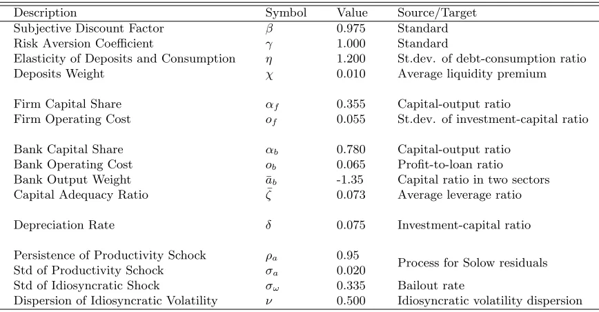
TABLE 1 : Configuration of Model Parameters . . . 57
TABLE 2 : First Aggregate Moments . . . 58
TABLE 3 : Second Aggregate Moments . . . 59
TABLE 4 : Business Cycle Correlations . . . 60
TABLE 5 : Optimal Bank Capital Policy (Benchmark Quantitative Model) . . 61
TABLE 6 : Optimal Bank Capital Policy (Quantitative Model with Liquidity Shocks) . . . 62
TABLE 7 : Asset Returns in the Data . . . 108
TABLE 8 : Asset Payouts in the Data . . . 109
TABLE 9 : Asset Payout Cyclicality . . . 110
TABLE 10 : Wavelet Correlation between Asset Payout and Consumption Growth111 TABLE 11 : Configuration of Model Parameters . . . 112
TABLE 12 : Model Implications: Consumption . . . 112
TABLE 13 : Model Implications: Asset Payouts . . . 113
TABLE 14 : Model Implications for Asset Prices . . . 114
TABLE D.1 : Barclays Index Data . . . 132
TABLE E.1 : Equity Payout Cyclicality . . . 135
TABLE E.2 : Debt Payout Cyclicality . . . 136
LIST OF ILLUSTRATIONS
FIGURE 1 : Rate of Return on Deposits . . . 47
FIGURE 2 : Socially Optimal Allocation . . . 48
FIGURE 3 : Competitive Equilibrium Allocation . . . 49
FIGURE 4 : Effects of Capital Regulations on the Bank’s Lending Costs . . . 50
FIGURE 5 : Lending Capital Requirement . . . 51
FIGURE 6 : Exogenous TFP Shock. . . 52
FIGURE 7 : Exogenous TFP Shock. . . 53
FIGURE 8 : Exogenous Liquidity Shock. . . 54
FIGURE 9 : Exogenous Liquidity Shock. . . 55
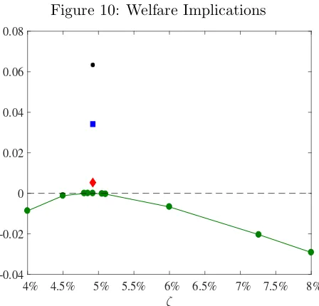
FIGURE 10 : Welfare Implications . . . 56
FIGURE 11 : Debt Market Capitalization . . . 96
FIGURE 12 : Asset Market Capitalization . . . 97
FIGURE 13 : Equity, Debt, and Asset Payouts . . . 98
FIGURE 14 : Changes in Equity, Debt, and Asset Payouts . . . 99
FIGURE 15 : Term Structure of Payout Cyclicality (Consumption) . . . 100
FIGURE 16 : Term Structure of Payout Cyclicality (Output) . . . 101
FIGURE 17 : Term Structure of Return Cyclicality . . . 102
FIGURE 18 : Change in Debt Payouts: Book and Market Values . . . 103
FIGURE 19 : Term Structure of Payout Cyclicality: Book Values of Debt . . . 104
FIGURE 20 : Term Structure of Equity Payout Cyclicality: 1975-2014 . . . 105
FIGURE 22 : Model Implications for Payout and Return Cyclicality . . . 107
FIGURE E.1 : Term structure of Asset Payout Cyclicality: Global Risks . . . . 134
FIGURE E.2 : Term structure of Asset Cash Payout Cyclicality: Normalized Changes
CHAPTER 1 : DYNAMIC BANK CAPITAL REQUIREMENTS
1.1. Introduction
The recent financial crisis imparted renewed attention on the stability of the banking sector
and on capital regulation. Both policymakers and academics have recognized that
risk-based capital requirements, such as those in the 2004 Basel II Accord, tend to exacerbate
business-cycle fluctuations, leading to an overly cyclical credit supply. To protect the
bank-ing sector from periods of excess credit growth and leverage buildup, the 2010 Basel III
Accord introduced the countercyclical capital buffer (CCyB) framework. The proposed
adjustment effectively translates into capital ratios that vary over time. Despite a few
re-cent trials to implement CCyB regimes within countries in the European Union, there is
no consensus at the practical or theoretical level about the implications of CCyBs on the
macroeconomy1.
The goal of this paper is to investigate both the theoretical and quantitative implications
of optimal state-dependent capital requirements. By comparison, most of the existing
lit-erature has limited itself to examining the costs and benefits of the overall level of capital
requirements.2 To this end, I develop a tractable general equilibrium model and use it to
characterize optimal bank capital requirements. The problem of choosing an optimal capital
policy follows from the work of Ramsey (1927) and builds on the primal approach used in
the optimal taxation literature3.
My model has three key features. First, high-quality production projects are scarce,
espe-cially during economic downturns. Second, banks benefit from government guarantees in
1
The expectation is that the buffer will be at zero through most of the business cycle and increase to the maximum 2.5% points only at the peak of the credit cycle. Even though under 2010 Basel Accord the CCyB regime will be phased in globally between 2016 and 2019, individual EU members have already introduced the CCyBs. For instance, the Bank of England maintained the buffer rate equal to 0% starting from 26 Jun 2014, and plans to increase it to 0.5% starting from 27 Jun 2018.
2
Some examples include Diamond and Rajan (2000), Diamond and Rajan (2001), Hellmann et al. (2000), Repullo (2004), Morrison and White (2005), Van den Heuvel (2008), Admati et al. (2010), DeAngelo and Stulz (2013), Nguyen (2014), Begenau (2016),
3
the form of bank bailouts, which lowers their borrowing cost, thereby creating incentives to
risk-shift. Third, households value money-like assets in the form of bank debt. This implies
that bank debt is priced at a premium and is a cheaper source of funding than equity. The
last two features create a trade-off: while tighter capital ratios can help to mitigate a bank’s
motives to risk-shift and rule out inefficient lending, at the same time they can reduce the
bank’s supply of credit and the creation of safe liquid assets4.
In the model, procyclical capital requirements (or, equivalently, countercyclical capital
buffers) emerge endogenously as an optimal policy scheme in a Ramsey equilibrium.
Be-cause of government guarantees, banks end up financing low-quality projects and more so
during periods of high economic growth, even though they are inefficient from the social
prospective. The reasons are twofold. Because of better lending opportunities during
ex-pansions, banks increase the supply of credit and deposits. As a result, the premium on
band debt becomes smaller, thereby increasing the value of default option and lowering the
banks borrowing costs. This translates into an even higher level of lending. In addition,
during expansions banks risk-shift on a larger scale, which implies that more inefficient
projects are financed in absolute terms. Consequently, heightened capital regulation can
be most beneficial through credit booms. At the same time, tight capital requirements can
have a contractionary effect on bank activity especially during recessions, when liquidity is
most valuable to households and, as a result, equity financing is more costly for banks. This
implies that optimal capital charges should be lower during economic slowdowns, thereby
reinforcing the cyclicality of optimal capital ratios.
In the model, procyclical capital requirements (or, equivalently, countercyclical capital
buffers) emerge endogenously as an optimal policy scheme. Presence of government
in-duces banks to finance low-quality production projects, even though they are inefficient
from the social prospective. My results show that investment in such projects builds-up
4
during periods of high economic growth. Because of better lending opportunities during
expansions, banks increase the supply of credit. As a result, expected bailout subsidies
become larger, thereby lowering banks borrowing costs and translating into an even higher
level of lending. Consequently, heightened capital regulation can be most beneficial through
credit booms. At the same time, tight capital requirements can have a contractionary effect
on bank activity especially during recessions, when liquidity is most valuable to households.
As banks reduce their deposit creation during downturns, the premium on bank debt
in-creases and, as a result, equity financing becomes more costly for banks.5 This implies that
optimal capital charges should be lower during economic slowdowns, thereby reinforcing the
cyclicality of optimal capital ratios.
In the model, procyclical capital requirements (or, equivalently, countercyclical capital
buffers) emerge endogenously as an optimal policy scheme. Because of government
guaran-tees, banks end up financing low-quality production projects, even though they are inefficient
from the social prospective. My results show that investment in such projects builds-up
during periods of high economic growth, when the bailout wedge – expected government
subsidy – is large. In the model, both the size of the government transfer and probability of
receiving it increase in bank level of lending. As banks issue more loans, they move further
into the distribution of projects’ quality and, thus, lower the quality of a marginal loan
on their balance sheet. Because of better lending opportunities during expansions, banks
increase the supply of credit. As a result, expected bailout subsidies become larger, thereby
lowering bank borrowing costs and translating into an even higher level of inefficient lending
during expansions. This implies that heightened capital regulation can be most beneficial
through credit booms. At the same time, tight capital requirements can have a
contrac-tionary effect on bank activity especially during recessions, when liquidity is most valuable
to households. As banks reduce their lending and deposit creation during downturns, the
5
premium on bank debt increases and, as a result, equity financing becomes more costly for
banks.6 Consequently, optimal capital charges should be lower during economic slowdowns,
thereby reinforcing the cyclicality of optimal capital ratios.
My results also show that the optimal Ramsey policy used as a single policy tool is not
sufficient to restore both the socially optimal level of lending and liquidity provision. To
provide some intuition behind the design of optimal capital regulations, I solve separately for
the “lending capital requirement” – restoring the first-best level of investment but admitting
a reduced level of deposits – and the “liquidity capital requirement” – ensuring the first-level
of liquidity provision but also allowing for excessive lending. Such policies focus only on one
dimension of the problem, either dampening incentives of banks to risk-shift or stimulating
creation of safe and liquid assets. By contrast, the Ramsey capital requirement balances
reduced inefficient lending with reduced liquidity provision.
The model highlights important trade-offs one needs to consider when regulating bank
capital. However, for effective policy making, it is also crucial to assess these trade-offs
quantitatively. I therefore calibrate the model to best match key macroeconomic quantities
and bank data variables. Using this choice of parameters, I solve numerically for the optimal
policy in the Ramsey equilibrium. Specifically, I characterize the optimal state-contingent
capital regulation and the set of allocations for bank lending and liquidity provision that
maximize consumers’ lifetime utility. Ramsey allocations have the property that they can
be implemented as a competitive equilibrium when banks encounter the prescribed capital
requirements. I find that the optimal Ramsey policy requires a cyclical capital ratio that
mostly varies between 4% and 6% and depends on key indicators of economic growth and
asset prices. This range of values is roughly comparable with a 2.5% upper bound of the
CCyB proposed by the Basel III Accord. Importantly, the optimal policy rule is not capped
at 6%, and can rise above it during periods of abnormal economic growth. In addition, the
6
mean Ramsey capital requirement is around 5%. This is one percentage point higher than
the level of the leverage ratio, and one percentage point lower than the Tier 1 capital ratio
as recommended by the Basel III Accord.
Implementing the optimal Ramsey policy delivers a permanent increase in the annual
con-sumption and deposit holdings of households relative to the average capital ratio observed
in the data. Although the exact magnitude of the welfare gain depends on the attitude
of households toward risk, more than 60% is attributed to having state-dependent capital
requirements. The remaining welfare improvement is achieved by setting an optimal fixed
capital requirement equal to the mean Ramsey capital ratio. The optimal policy leads to a
reduction in the cyclicality of bank credit – reducing inefficient lending during expansions,
but increasing the supply of credit during economic slowdowns – and, as a result, achieves
on average a higher level of consumption and deposit creation.
The main contribution of the paper is to characterize the optimal policy rule in terms of
measurable macroeconomic and bank aggregates. While the Basel Committee recommends
adjusting the capital requirements based on the “credit gap” – the deviation of the
credit-to-GDP ratio with respect to its long-term trend, – I show the credit gap alone fails to capture
the time variation in the optimal Ramsey policy. Instead, I find the optimal policy rule
takes into account the joint behavior of the credit gap, GDP, and the liquidity premium.
Specifically, the optimal policy is well approximated by the following rule:
capital ratio= 5% + 0.1%×credit gap+ 0.7%×GDP −0.1%×liquidity premium,
where the liquidity premium is a discount on the price of safe liquid assets.7 A one standard
deviation increase in the credit-to-GDP ratio (GDP) translates into a 0.1% (0.7%) increase
in capital charges, while a one standard deviation increase in the liquidity premium leads
to a 0.1% drop. Growth in bank credit, along with the output growth, act as indicators of
7The three indicators are expressed in log-deviations from their steady states and normalized by their
banks’ incentives to risk-shift. By contrast, the liquidity premium serves as an indicator of
how expensive equity financing is for banks and how valuable liquid assets are for investors.
The paper proceeds as follows: In Section 1.2, I provide the details of bank regulation,
as well as review the related literature. I develop the baseline model in Section 1.3. I
characterize the first-best allocation in this economy in Section 1.4, as well as the competitive
equilibria with and without capital regulations in place. In Section 1.5, I examine the lending
and liquidity capital requirements within the baseline model. I provide the quantitative
assessment of the model in Section 1.6, as well as present the optimal policy rule. Concluding
remarks are give in Section 1.7.
1.2. Bank Regulation and Related Literature
1.2.1. The Basel Accords
The Basel Accords, developed by the Basel Committee on Bank Supervision (BCBS),
con-solidate capital requirements as the cornerstone of bank regulation. The 1988 Basel Accord,
known as Basel I (BCBS (1988)), was criticized for the risk-insensitivity of capital charges.
To address this critique, the internal ratings-based (IRB) approach was introduced with
the publication of Basel II in 2004. Under risk-based regulation, the amount of capital
that a bank is required to hold against a given exposure depends on the estimated credit
risk of that exposure, which in turn is determined by the probability of default (PD), loss
given default (LGD), exposure at default (EAD), and maturity. The key implication of the
IRB approach is that riskier exposures carry a higher capital charge. The intention of this
approach is to reduce bank failures and the associated systemic costs by holding the bank
probability of default below some fixed target.
Both policymakers and academics have recognized that risk-sensitive capital regulations,
such as that in Basel II, tend to exacerbate the inherent cyclicality of bank lending and,
consequently, distort investment decisions. This is because in economics downturns losses
credit risk model, delivering higher capital charges. To the extent that it is difficult or costly
for a bank to raise new capital during recessions, it will be forced to cut back on its lending
activity. Kashyap et al. (2008) provide empirical evidence that equity-raising was sluggish
during the recent financial crisis.
Kashyap and Stein (2004) argue that the IRB approach is largely microprudential in nature
and ignores the importance of the function of bank lending. In line with the literature on
capital crunches in banking, they claim that the shadow value of bank capital increases
during recessions and a capital requirement that is too high when bank capital is scarce
may result in reduced funding of positive net present value projects. So, if the government’s
objective is both to protect the financial system against the costs of bank defaults and
sustain bank-lending efficiency, the capital charges should be adjusted to the state of the
business cycle (for any degree of credit-risk exposure).
An important argument that is sometimes made is that during periods of economic growth
banks may hold capital in excess of the minimum regulatory requirements that could
neu-tralize potential cyclicality problems. Repullo and Suarez (2012) develop a dynamic model
of relationship lending, in which banks hold voluntary capital buffers as a precaution. They
find that the capital buffers set aside during expansions are typically not sufficient to
pre-vent credit supply shrinkage during recessions. They also document that the optimal capital
requirements are higher and less cyclically-varying than the requirements of Basel II when
the social cost of bank failure is high.
In an attempt to strengthen bank balance sheets against future financial upheavals, Basel
III introduced the countercyclical capital buffers, which range from zero to 2.5% of
risk-weighted assets. As mentioned before, the BCBS proposed to adjust the level of the buffer
based on the credit gap, meanwhile acknowledging that it may not be a good indicator of
stress in downturns. For example, Repullo and Saurina (2011) find that the credit gap for
many countries is negatively correlated with GDP growth. This can be traced to the fact
Kashyap and Stein (2004), Gordy and Howells (2006), Saurina and Trucharte (2007), and
Kashyap et al. (2008), among others, focus on the correction of risk-based capital
require-ments in a macroprudential direction. Using Spanish data, Repullo et al. (2010) analyze
different procedures aimed at mitigating the procyclical effects of capital regulation and
conclude that the most appealing one is to use a business cycle multiplier based on GDP
growth. The proposed adjustment maintains the risk sensitivity in the cross-section (i.e.,
banks with riskier portfolios would bear a higher capital charge), but a cyclically-varying
scaling factor would increase capital requirements in good times and reduce them in bad
times. In line with this study, I propose a cyclical policy rule that depends positively on
indicators of economic growth. In my setting, state-contingent capital requirements emerge
endogenously as an optimal policy scheme. Optimal regulations promote the stability of
the banking sector without contracting the supply of bank credit and deposit creation.
Ar-guments in favor of time-varying capital regulations are also found in Kashyap et al. (2008),
Hanson et al. (2011), and Malherbe (2015). Note that I abstract from the cross-sectional
dimension of capital regulation and focus on the time-series dimension.
1.2.2. Literature Review
The most closely related paper is Malherbe (2015), which studies the optimal capital
re-quirement over the business and financial cycles. In his setting, because of the general
equilibrium effect and decreasing returns to scale in production a higher level of aggregate
banking capital calls for a tighter capital requirement to preclude inefficient credit growth.
Even though his model also finds that capital regulation should be tightened during boom
episodes, the mechanism is different from mine. Liquidity channel
This research project is at the intersection of a large literature on optimal banking
regu-lation theory and dynamic macroeconomic models of financial intermediation. The recent
financial crisis has brought to the forefront the discussion of whether the capital
require-ments of banks should be increased (Admati et al. (2010)). On one side, Hellmann et al.
regula-tion can induce prudent behavior by banks. On the other side, Diamond and Rajan (2000),
Diamond and Rajan (2001), and DeAngelo and Stulz (2013) provide theoretical evidence
that tightening capital requirements may distort banks’ provision of liquidity services, while
Dewatripont and Tirole (2012) show that stricter capital requirements may introduce
gover-nance problems. In line with the existing literature, I suggest that reduced moral hazard is
the key rationale for imposing restrictive capital regulation with reduced liquidity provision
being the main downside.
This paper is most closely related to other quantitative studies on the welfare impact of
capital requirements (Van den Heuvel (2008) , Nguyen (2014), Begenau (2016), Van den
Heuvel (2016)) and leverage constraints (Bigio (2010), Martinez-Miera and Suarez (2012),
Corbae and D’Erasmo (2014), and Christiano and Ikeda (2014) ). Among the most recent
studies estimating the optimal level of fixed capital requirements are Nguyen (2014) and
Begenau (2016). Nguyen (2014) finds that consumers’ lifetime utility is maximized at 8%
capital ratio, while the optimal number estimated by Begenau (2016) is 14%. A common
feature in these two papers is that government guarantees incentivize banks to engage in
excessive risk-taking, while capital regulation helps to address these distortions. Begenau
(2016) also extends the banks’ role to providing liquidity services, which are valued by
households. I complement this branch of literature by developing a tractable framework to
quantify the benefits and costs of capital regulation over the business cycle. This allows
me to provide not only qualitative, but also quantitative recommendations on the policy
design. To the best of my knowledge, this paper is the first to solve for the stage-contingent
capital requirements within the Ramsey framework.
My paper is closely related to the papers estimating an optimal level of fixed capital
re-quirement in a dynamic general equilibrium setting. In this sense, the paper complements
existing quantitative studies on the welfare impact of leverage constraints. Van den Heuvel
(2008) was one of the first to study the welfare cost of capital requirements in a
regulation dampens the ability of banks to create liquidity, leading to a welfare loss, and,
therefore, concludes that it is too high. In his paper the bank capital structure is recovered
from binding capital requirements and it is difficult to infer the welfare costs of alternative
levels of bank regulation than the current one. Among the most recent studies estimating
the optimal capital requirements are Nguyen (2014) and Begenau (2016). Nguyen (2014)
finds that the welfare is maximized at 8% capital ratio, while the optimal number
esti-mated by Begenau (2016) is equal to 14%. A common feature in these two papers is that
government guarantees incentivize banks to engage in excessive risk-taking, while capital
regulation helps to address these distortions. Begenau (2016) also extends the banks’ role
to providing liquidity services, which are valued by households.
My paper is also related to prior contributions focused on welfare implications of capital
constraints. Corbae and D’Erasmo (2014), Christiano and Ikeda (2014), Bigio (2010) and
Martinez-Miera and Suarez (2012) reach the conclusion that a tighter leverage constraint
lowers the riskiness of the financial sector, but that it also shortens bank lending capacity,
thereby depressing the economic growth. Corbae and D’Erasmo (2014) study the
quanti-tative impact of capital regulation on bank risk-taking, bank failures and market structure
when there is competition among small and big banks. Bigio (2010) develops a model with
endogenous liquidity mechanism and analyzes how capital requirements change the risk
capacity of the economy. Christiano and Ikeda (2014) quantify the effects of leverage
con-straints in a framework where bankers have an unobservable effort choice. Martinez-Miera
and Suarez (2012) study the role of banks in generating systemic risk taking and find that
optimal capital requirements are quite high and don’t require counter-cyclical adjustments.
This is one of the first paper which looks at the welfare implications of time-varying capital
regulation.
There are few empirical contributions on the effects of higher capital requirements on bank
lending and bank cost of capital. Looking at the data on large financial institutions, Kashyap
loan rates is likely to be modest, in the range of 25 to 45 bps. In a similar vein, Baker and
Wurgler (2013) calibrate that a ten-percentage point increase in capital requirements would
translate into a higher weighted average cost of capital by 60-90 bps per year. Kisin and
Manela (2013) estimate the perceived costs of capital requirements by employing the data
on banks’ participation in a costly loophole that helped them to bypass capital regulations.
They document that a ten-percentage point increase in Tier 1 capital to risk-weighted assets
leads to, at most, a 3 bps increase in banks’ cost of capital. Even though these studies shed
light on the potential impact of capital regulations on the real economy, it is difficult to
assess the overall welfare implications of a time-varying capital requirement in their setting.
More broadly, this paper fits a strand of macroeconomic literature on the role of financial
intermediation in the development of economic crises. The transmission mechanism by
which the effects of small shocks persist, amplify, and spread to the macroeconomy is first
identified in the seminal works of Bernanke and Gertler (1989), Kiyotaki and Moore (1995),
and Bernanke et al. (1999). The more recent studies of the balance sheet channel include
Gertler and Kiyotaki (2010), Gertler and Karadi (2011), He and Krishnamurthy (2012),
Di Tella (2013), and Brunnermeier and Sannikov (2014).
1.3. Model Setup
To focus on the novel mechanisms associated with dynamic bank capital requirements, I
first layout the baseline model, which is kept as parsimonious as possible. I later augment
the model to quantify policy recommendations on what defines optimal time variation in
capital requirements of banks.
I develop a model studying the welfare implications of an endogenous capital requirement.
Government guarantees can introduce distortions in bank incentives and lead to excessive
risk-taking in equilibrium. Socially optimal allocation - both the first-best level of lending
and first-best level of liquidity provision - can not be restored with help of only one policy
time-varying capital requirement.
In the model, time is discrete and runs for an infinite number of periods. Financial
interme-diaries own the production technology and the stock of capital in this economy. They are
financed either partially or entirely with deposits. The presence of deposit insurance
dis-torts banks’ optimal choices of investment. Households consume the final goods produced
in the banking sector and invest any savings in the banks’ deposits. To finance bailout
expenditures, the government levies taxes on households in lump-sum fashion.
1.3.1. Banking Sector
I start by characterizing a banking sector in detail. At any point in time the economy is
populated with a continuum of ex ante identical banks of measure one, indexed byj∈Ω =
[0,1]. Each bank has access to decreasing returns to scale technology and produces a final
goodyj,t, using capital as the only input,
yj,t =eωj,t+atlαj,t,
whereat is an aggregate productivity shock, which follows:
at= (1−ρa) ¯a+ρaat−1+σat, t∼iidN (0,1) (1.1)
and ωj,t is an idiosyncratic disturbance, which is identically distributed across time and across banks:
ωj,t=− 1 2σ
2
ω+σωεj,t, εj,t ∼iidN (0,1). (1.2)
In the cross-section, the bank-specific shocks average to zero. This setup is isomorphic
to the one, where a consumption good is produced by penniless firms, who have been
credit rationed in the capital markets due to unmodeled information asymmetries, and
whose only source of funding is bank loans.8 The capital used in banks’ production process
8Suppose that each bank operates on an islandj; one can think of an island as an industry or a state.
can be correspondingly interpreted as the amount of bank loans issued to these types of
borrowers. From this point on, I refer to lj,t+1 as bank lending. The decreasing returns
to scale assumption is crucial to capture the idea that borrowers are not homogeneous and
that there is a finite number of creditworthy borrowers, or equivalently a finite number
of positive net present value (NPV) production projects. This setup ensures that banks
internalize that each extra lending unit (borrower) is not as productive (creditworthy) as
the previous one.
A bank j enters a period twith capital, lj,t, bank debt, dj,t, and equity, nj,t. The balance sheet equates risky assets, lj,t, to bank debt,dj,t, and equity,nj,t:
Bankjenters periodtwithlj,t lending units, financed with dj,t units of debt and nj,t units of equity. The balance sheet equates risky assets to bank debt and equity:
lj,t – loans nj,t – net worth dj,t – debt
The bank’s revenues realized at time t are equal to its earnings on the production net of
the interest payments on its liabilities:
πj,t =eωj,t+atlαj,t−lj,t−(Rd,t−1)dj,t.
For the statement of problem, it is useful to define equity after profits as ˜nj,t≡πj,t+nj,t.
Next, I assume that when a financial intermediary does not have sufficient funds to service
at timet+ 1. Firms on each island are ranked according to their productivity. Specifically, a firmion an islandj(whereidenotes the firm’s ranking) producesαeωj,t+atiα−1 units of a consumption good. At time t, the bank on islandjissues loans to the firstlj,t+1firms with the total amount equal to:
Z lj,t+1 0
1di=lj,t+1.
The monopolist bank on the island can extract all surplus. In particular, at timet+ 1 the bank on islandj
receives from the firms:
Z lj,t+1 0
its deposit liabilities, depositors are bailed out with probability one.9 In particular, banks
will default on their credit obligations whenever their idiosyncratic shock ωj,t is below a cutoff levelωj,t∗ , defined by the expression:
πj,t+nj,t= 0⇔eω
∗ j,t+atlα
j,t=Rd,tdj,t.
The net worth, nj,t+1, available to banks at the end of period t (going into period t+ 1),
evolves according to:
nj,t+1={πj,t+nj,t}+−zj,t (1.3) =neωj,t+atlα−1
j,t −Rd,t
lj,t+Rd,tnj,t
o+
−zj,t,
where{·}+ denotes the maximum operatormax{·,0}and captures that banks are subject
to limited liability and government guarantees. zj,t is the net payouts to the bank’s share-holders. A positive net transfer, zj,t >0, means that the equityholders receive dividends, while a negative one,zj,t<0, means that there is an equity issuance. Equation 1.3 demon-strates that any growth in bank equity above the deposit return depends on the premium
that the financial intermediary earns on its assets, as well as the total amount of lending. To
finance the difference between the capital investment and available net worth, the financial
intermediary borrows an amount dj,t+1 from households, given by:
dj,t+1=lj,t+1−nj,t+1.
Finally, banks are subject to capital regulations, which require them to have a minimum
9
amount of equity as a fraction of assets. Since loans are the only type of asset in my model,
the capital requirement I instate is that equity needs be at least a fraction ζt of loans for a bank to be able to operate:
nj,t+1 ≥ζtlj,t+1.
In each period, bankj decides how many loans to issue,lj,t+1, and makes a leverage choice
to maximize the discounted sum of the equity payouts:
max zj,t,lj,t+1,dj,t+1,nj,t+1
E " ∞
X
t=0
βtzj,t
#
(1.4)
s.t. nj,t+1=
eωj,t+atlα
j,t−Rd,tdj,t +−zj,t, lj,t=nj,t+dj,t,
nj,t+1≥ζtlj,t+1,
nj,0, dj,0 given.
makes an investment choice - how much loans to issue,lj,t+1, and a leverage choice - with how
much debt, dj,t+1, and how much equity, nj,t+1, to finance their investment - to maximize
the expected payouts to shareholders.
1.3.2. Household Sector
The economy is populated by a measure one of identical households. There are two types of
members in each household: savers and bankers (Gertler and Karadi (2011)). Savers hold
deposits at a diversified portfolio of financial institutions and return the interest earned to
their household. Bankers, on the other hand, manage financial intermediaries and similarly
return any earnings back to the household. The savers hold deposits at the banks that
its household does not own, otherwise in the absence of tax frictions, the Modigliani-Miller
theorem would hold and the irrelevance of banks’ capital structure would follow. Savers’ and
agent framework.
LetCt denote family consumption andDt+1 denote the holdings of bank deposits.
House-holds are risk-neutral and have a discount rate ofβ∈(0,1).10I also assume that households
value the non-pecuniary services provided by bank deposits and, hence, enjoy the additional
flow of utilityv(Dt+1), which is a concave non-decreasing function of the supply of deposits
Dt+1.11
Then households preferences are, therefore, given by
u(Ct, Dt+1) =Ct+ D1t+1−η
1−η, η <1.
In each period, the household chooses a consumption level and deposit holdings to maximize
their utility subject to the budget constraint:
max Ct,Dt+1
E "∞
X
t=0
βt(Ct+v(Dt+1))
#
(1.5)
with v(Dt+1) =
D1t+1−η
1−η, η <1
s.t. Ct=Rd,tDt−Dt+1+Zt−Tt, D0 given,
whereTtis a lump-sum tax levied by the government. Households are the owners of financial intermediaries and at the end of each period receive the net proceeds of bank activity, Zt. A unit of deposits issued in period tyields a gross return of Rd,t+1 at timet+ 1.
The presence of the government guarantees implies that Rd,t+1 is a return on a riskless 10
A household’s consumption can be both positive and negative, as in Brunnermeier and Sannikov (2014). Negative consumption can be interpreted as disutility from labor.
11
asset. The first-order conditions of 1.5 impart that the interest rate on deposits is equal to:
Rd,t+1 =
1 β −
1 βD
−η t+1.
| {z }
liquidity premium
(1.6)
Since households exhibit a preference for bank debt, there is a discount on its interest rate,
which is the amount households are willing to relinquish in exchange for holding a risk-free
asset, which gives a flow of utility compared to a risk-free asset that does not give a flow
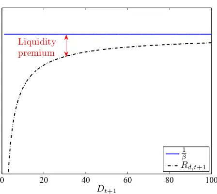
of utility.12 Figure 1 shows that liquidity premium is a decreasing function in the supply
of bank deposits. This implies that liquid deposits become more valuable to the household
when they are scarce.
Diamond and Dybvig (1983) were among the first to analyze household demand for
liq-uidity. They find that bank deposits provide better risk-sharing possibilities to consumers,
justifying the existence of the liquidity premium. Stein (2011) and Gorton and Metrick
(2012) argue that collateralized short-term debt issued by banks yields a “money-like”
con-venience premium based on its relative safety and the transactions services that safe claims
provide. Further, Krishnamurthy and Vissing-Jorgensen (2012) and Krishnamurthy and
Vissing-Jorgensen (2015) document that investors value the money-like features of
Trea-suries the most, when the supply of TreaTrea-suries is low. The welfare implications of the
presence of liquidity premium via its effects on the lending costs of banks have also been
studied by Begenau (2016) and Van den Heuvel (2016).
1.3.3. Government
The role of the government is to provide deposit insurance. To finance its expenditures on
bank bailouts, the government levies a lump-sump tax on households in accordance with a
12
In this setting, the rate of return on any other safe asset other than bank debt is equal to β1. As long as households derive utility from bank deposits and the economy is not fully saturated with liquidity, the interest rate on bank debt is always lower than the interest rate on any other risk-free asset,
lim
Dt+1→∞
Rd,t+1=
1
balanced budget rule:
Tt=
Z 1
0
max
Rd,tdj,t−eωj,t+atlαj,t,0 dj. (1.7)
1.4. Equilibrium Characterization
Definition. A competitive equilibrium is a set of prices {Rd,t+1}∞t=0, government policies
{ζt, Tt}∞t=0, and allocations
n
Ct, Dt+1,{zj,t, lj,t+1, nj,t+1, dj,t+1}j∈Ω
o∞
t=0, such that:
(i) Given prices {Rd,t+1}∞t=0, government policies {Tt}∞t=0 and initial amount of savings, D0, households maximize their life-time utility given by 1.5;
(ii) Given prices{Rd,t+1}∞t=0, government policies {ζt, Tt}∞t=0 and initial capital structure {nj,0, dj,0}j∈Ω, each bankj∈Ω maximizes the discounted sum of equity payouts given
by 1.4;
(iii) The government budget constraint 1.7 is satisfied;
(iv) Market clearing conditions hold:
– resource constraint
Ct+
Z 1
0
lj,t+1dj =
Z 1
0
yj,tdj,
– deposits market
Dt+1=
Z 1
0
dj,t+1dj.
The nature of the bank’s problem 1.4 implies that the equilibrium is symmetric and all banks
make identical decisions. The realization of the bank-specific shock ω induces a bailout
transfer from the government to a subgroup of banks, but does not affect the optimal
shareholders as follows:
J(lj,t, nj,t, ωj,t, St) =max{πj,t+nj,t,0}+V (St),
where the continuation valueV (·) obeys the following Bellman equation:
V (St) = max nj,t+1,lj,t+1
−nj,t+1+Et
βMt,t+1 Z +∞
0
J(lj,t+1, nj,t+1, ωj,t+1, St+1)dF(ωj,t+1)
(1.8)
= max
nj,t+1,lj,t+1
(
−nj,t+1+Et
"
βMt,t+1
Z +∞
ω∗
j,t+1
(πj,t+1+nj,t+1)dF(ωj,t+1) +V(St+1)
!#) .
The conditional expectationEtis taken only over the distribution of aggregate productivity shocks andSt denotes the aggregate state of the economy. To the extent that bank-specific shocks are not persistent and there is no equity issuance costs, all financial intermediaries are
ex ante the same and make identical decisions. In particular,lj,t+1 =Lt+1, nj,t+1 =Nt+1,
and dj,t+1=Dt+1,∀j∈Ω.
To uncover the inefficiencies introduced with the presence of government subsidies, I first
solve for the socially optimal allocation in this economy. Next, I characterize a competitive
equilibrium when banks face no capital regulations and then compare the optimal decisions
of banks in the two equilibria.
1.4.1. First-Best Allocation
A social planner chooses consumption and supply of liquid deposits to maximize households’
lifetime utility subject to the resource constraint:
max Ct,Lt+1,Dt+1≤Lt+1
E "∞
X
t=0
βt Ct+ D1t+1−η 1−η
!#
(1.9)
where the regulator takes into account that the competitive equilibrium is symmetric and
that the deposit’s supply is bounded by the stock of capital in the banking sector. I
characterize the socially optimal allocation in Proposition 1.
Proposition 1 The first-best allocation is characterized by:
(i) Bank’s optimal finance policy:
DF Bt+1 =LF Bt+1, NtF B+1 = 0.
(ii) Optimal level of bank lending, LF B
t+1, defined by:
Et
Rl,tF B+1
=Rd,tF B+1 (1.10)
with
RF B
l,t+1 =αeat+1 LF Bt+1
α−1
and RF B d,t+1 =
1 β −
1 β D
F B t+1
−η .
Proposition 1 follows directly from the first order conditions to 1.9. The proofs of all
propositions are given in Appendix A. Because households value money-like securities, it
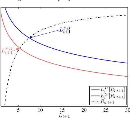
is optimal to finance all bank production with debt. The expression 1.10 pins down the
first-best level of lending by equating the marginal productivity of bank capital stock to the
marginal cost of lending (Figure 2). The social marginal cost of funding is equal to the rate
of return at which a household is willing to hold deposits at the financial intermediaries,
RF B
d,t+1. It seems implausible that the social planner would find it optimal not to keep any
equity on the bank’s balance sheet. As an extension, I can introduce the social cost of bank
default. In such a setup, the optimal level of a bank net worth,NF B
t+1 >0, would trade off
reduced liquidity provision and reduced social cost of bank default.
I interpret the first-best level of lending,LF B
t+1, as an upper limit on the amount of positive
that there are fewer good lending opportunities during economic slowdowns than during
expansions, as I state in Proposition 2.
Proposition 2 The socially optimal level of lending, LF B
t+1, is procyclical:
∂LF B t+1
∂at >0.
Proposition 2 is established using the equilibrium condition 1.10 and an implicit function
theorem (see Appendix A). Since the marginal productivity of lending is higher in good
times, when the marginal cost is acyclical (Figure 2), it is optimal to maintain a higher level
of production during expansions. This naturally advocates for a less stringent government
regulations during periods of economic growth, when there are more lending opportunities.
1.4.2. Competitive Equilibrium with No Capital Regulation
To highlight the economic mechanism at the heart of the model, I now provide a detailed
characterization of the bank’s lending and capital structure choice in a competitive
equi-librium. In this section, suppose that financial intermediaries face no capital regulation or,
equivalently,ζt= 0,∀t.
The banks’ first order conditions with respect to lending and the amount of equity financing
are, respectively, given by:
Et[Rl,t+1] =Rd,t+1−Et
" Z ω∗t+1
0
(Rd,t+1−eωRl,t+1)dΦ (ω)
#
, (1.11)
−
1
β −Rd,t+1
−Et
" Z ω∗t+1
0
Rd,t+1dΦ (ω)
#
<0, (1.12)
where the implicit (aggregate) rate of return on loans is equal toRl,t+1 =αeat+1Lαt+1−1 and
the bailout threshold is defined byeωt∗+1+at+1Lα
t+1 =Rd,t+1(Lt+1−Nt+1). Φ (·) denotes the
normal distribution with mean −1
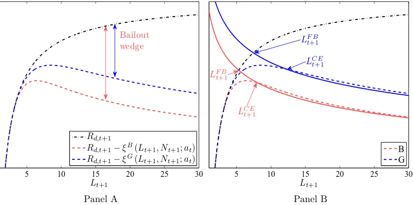
The presence of government guarantees generates a bailout wedge in the bank’s cost of
lending, defined by:
ξ(Lt+1, Nt+1;at)≡Et
" Z ω∗t+1
0
(Rd,t+1−eωRl,t+1)dΦ (ω)
#
.
This bailout wedge captures the difference between the social and private marginal cost of
lending (see equations 1.10 and 1.11). The bank does not fully internalize the risk costs,
since those are partially borne by the taxpayers. In particular, whenever the bank’s profits
are hit by a sufficiently low idiosyncratic shockω < ω∗t+1, their credit liabilities are covered by the government. An important property of the bailout wedge is that for a given level
of lending it is decreasing in the aggregate productivity,∂ξ/∂at<0 (Panel A of Figure 3). The economy is less likely to transition to a recession next period if it is currently in an
expansion, implying a lower bailout wedge during periods of economic growth.
Similarly, I can show that the bailout wedge is decreasing in Nt+1. The more net worth
financial intermediaries are holding on their balance sheet, the safer they are, the less likely
they will be bailed out and, hence, the smaller is the wedge in the lending cost.
The expression 1.12 demonstrates that equity is relatively a more expensive source of funding
for banks than debt. The reasons for this are twofold. By holding equity on their balance
sheets, banks forgo government subsidies and, at the same time, relinquish the liquidity
premium. As a result, the financial intermediaries will tilt their capital structure towards
debt and hold no equity on their balance sheets.
The funding wedge is strictly positive ξ(Lt+1, Nt+1;at) > 0, implying that the social
marginal cost of lending is strictly greater than the private one. Therefore, there exists an
excessive lending in a competitive equilibrium when the banks face no capital regulations,
LCE
t+1> LF Bt+1.13 It is a well documented in the banking literature, that government
guaran-tees incentivize banks to risk-shift. Contrary to the literature, in my model banks risk-shift
13
in terms of quantity, rather than in terms of quality. By issuing more loans, banks move
further into the distribution of the projects’ quality (borrowers’ creditworthiness), meaning
that more loans result in a lower quality loan portfolio. I lay out a characterization of the
competitive equilibrium in Proposition 3.
Proposition 3 The competitive equilibrium with no capital regulation in place is
charac-terized by:
(i) Optimal level of lending,LCE
t+1, defined by:
Et
RCEl,t+1
=RCEd,t+1−ξ LtCE+1, NtCE+1;at
, (1.13)
with
RCEl,t+1 =αeat+1 LCE
t+1
α−1
and RCEd,t+1 = 1 β −
1 β D
CE t+1
−η .
(ii) Bank’s optimal finance policy:
DCEt+1 =LCEt+1 > LF Bt+1, NtCE+1 =NtF B+1 = 0.
In the competitive equilibrium with the risk-shifting mechanism in place, the optimal level
of lending continues to be pro-cyclical (see Proposition 4). On the one side, lending is more
productive during expansions, calling for a higher level of investment. On the other side,
bank cost of lending goes up in good times because of a reduced bailout wedge, pushing the
optimal level of lending down (Panel B of Figure 3). Under log-normality of the aggregate
productivity shock, the former channel dominates the later and, hence, the procyclicality
of the optimal level of lending follows.
Proposition 4 In a competitive equilibrium with no capital regulations in place, the optimal
level of lending is procyclical:
∂LCE t+1
Using capital regulations, the government will aim to restrict inefficient lending that arises
in a competitive equilibrium. And whether tight capital requirements will be more
benefi-cial during expansions or recessions will depend on how the level of excessive investment,
LCE
t+1/LF Bt+1−1, behaves over the business cycle. Proposition 5 provides the condition under
which the lending level in a competitive equilibrium is more procyclical than the first-best
allocation.
Proposition 5 The level of overinvestment is procyclical if and only if
−ξ¯a,t<
∂ξ LCE
t+1, NtCE+1;at
∂at
<0. (1.14)
The threshold value ¯ξa is defined in Appendix A. There are a number of channels in force that indicate how banks’ risk-shifting incentives change over the business cycle. First, a
decreasing returns to scale production technology generates a scale effect: in proportionate
terms banks risk-shift, by the same amount across the states of the economy, but since in
good times they risk-shift on a larger scale, the overinvestment is higher in absolute terms.
This mechanism can be demonstrated in the setup in which the bailout wedge is
proportion-ate to the deposit rproportion-ate and the deposit rproportion-ate is constant. The second channel arises due to
the fact that the value of default option (or, equivalently, bailout option) increases during
periods of economic growth as banks’ liabilities to debtholders become larger. Since during
good times the economy is more saturated with deposits, households are willing to
relin-quish a smaller premium on safe assets, delivering a higher deposit rate. This property of
the default option results from the concave preferences for liquid assets and can be
demon-strated in the setup in which banks have a constant returns to scale production technology.
Third, assuming everything else is equal, the probability of exercising the default option
is decreasing in the productivity shock at, meaning that the amount of inefficient lending is reduced in good times. The restriction 1.14 ensures that in the equilibrium the banks’
The second channel arises due to the fact that the bailout wedge is increasing in lending,
∂ξ/∂Lt+1 > 0, as shown in Panel A of Figure 3. The more loans that banks issue, the
bigger is the size of the government transfer in case a bailout happens. This property
of the bailout wedge results from the concave preferences for liquid assets and decreasing
returns to scale in production. On the one side, a higher level of investment during periods
of economic growth implies a higher deposit rate, since the economy is saturated with
deposits and households are willing to relinquish a smaller premium on safe assets. On the
other side, decreasing returns to scale imply a lower income that is forgone in a bailout
when banks increase lending. A higher deposit rate and a lower rate of return on loans,
in turn, deliver a larger bailout wedge during expansions. Third, assuming everything else
is equal, the bailout wedge is decreasing in the productivity shock at, meaning that the amount of inefficient lending is reduced in good times. The restriction 1.14 ensures that
in the equilibrium the bailout wedge or, equivalently, the banks’ risk-shifting motives are
procyclical.
1.4.3. Competitive Equilibrium with Capital Regulation
Next suppose that equity needs be at least a fractionζt>0 of loans for banks to be able to operate. Given that in my model equity is a relatively more expensive form of finance for
banks than debt, the capital constraint is binding in each period of time (see Proposition
6).
Proposition 6 The capital constraint is binding:
NtCE+1 =ζtLCEt+1, DCEt+1= (1−ζt)LCEt+1.
To demonstrate what are the implications of capital regulation on bank cost of lending, I
equity financing, respectively, given by:
Et
RCEl,t+1
=RCEd,t+1−ξ LtCE+1, NtCE+1;at
+ 1 βλtζt, | {z }
equity wedge
(1.15)
1
βλt=Et "
Z ω∗
0
RCEd,t+1dF(ω)
#
+
1 β −R
CE d,t+1
, (1.16)
where λt is a Lagrange multiplier on the capital constraint. Imposing capital regulation introduces an equity wedge into the bank’s cost of funding. The first term of equation 1.16
captures that a better capitalized bank forgoes the government subsidies and, as a result,
faces higher lending costs. A positive level of capital requirement also means that the bank’s
supply of deposits is reduced, implying a higher liquidity premium and, as a result, a higher
equity wedge, as captured by the second term of equation 1.16.
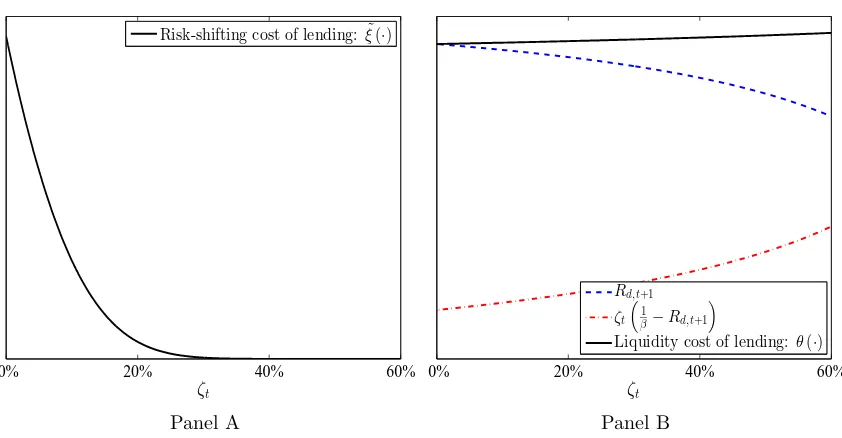
To better understand the costs and benefits of capital regulation, it is useful to decompose
the bank’s funding costs into (i) the liquidity channel and (ii) the risk-shifting channel,
which are, correspondingly, defined by:
θ(Lt+1, ζt)≡Rd,t+1+ζt
1
β −Rd,t+1
,
˜
ξ(Lt+1, ζt;at)≡Et
" Z ω∗t+1
0
((1−ζt)Rd,t+1−eωRl,t+1)dΦ (ω)
#
.
The obvious benefit of tightened capital requirements is reduced risk-shifting incentives
for banks. As shown in Panel A of Figure 4, the bailout wedge adjusted for the
pres-ence of capital regulations ˜ξ decreases as capital regulations are tightened, implying that
less inefficient firms are financed. There are two reinforcing mechanisms in place: the
bailout thresholdω∗t+1, as well as the size of a government transfer in case of a bank failure ((1−ζt)Rd,t+1−eωRl,t+1), falls as capital requirements become more stringent.
The level of the liquidity costs of lendingθis mainly determined by the amount of deposits
is reduced and, as a result, a liquidity premium is magnified. From the bank’s perspective,
this implies a lower required rate of return on debt, but a higher equity wedge (Panel B
of Figure 4). As long as η < 1, the liquidity cost of lending is strictly increasing in ζt. Overall, capital regulations translate into a heightened lending costs for banks, suggesting
that excessive lending can be restrained by imposing a sufficiently high capital requirement.
1.4.4. Optimal Capital Requirements
The goal of a social planner when choosing an optimal level of capital requirements is to
dampen bank’s risk-shifting incentives, but without restricting the bank’ supply of
high-quality loans and deposits. As a matter of fact, it is not feasible to restore both first-best
level of lending and liquidity provision at the same time with only the help of capital
requirements. Suppose for now that the only goal of the regulator is to restore a socially
optimal lending level and to achieve this goal the capital requirement is set toζL
t >0, which is the “lending capital requirement”. This translates into a level of liquidity provisionDtζ+1L that is below the socially optimal lending level:
Dζt+1L = 1−ζtL
LF Bt+1< LF Bt+1 =DF Bt+1.
Similarly, consider a social planner who aims to recover a socially optimal level of deposits
and imposes a capital requirement of ζD
t , which is the “liquidity capital regulation”. This capital requirement, however, allows inefficient lending from a social perspective:
Lζt+1D = D ζD
t+1
1−ζD t
= L F B t+1
1−ζD t
> LF Bt+1.
To provide the intuition behind the design of the optimal capital regulations, I first solve
for the lending and liquidity capital requirements in the baseline model. This allows me to
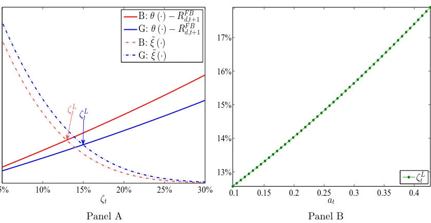
Lending Capital Requirement
Suppose now that the only goal of the social planner is to rule out excessive bank lending.
To do so, she institutes the lending capital requirement, defined in Proposition 7.
Proposition 7 The first-best level of bank lending,Lζt+1L =LF B
t+1, is restored when a capital
requirement is set to ζL
t , defined by:
θ LF Bt+1, ζtL
−RF Bd,t+1 = ˜ξ LF Bt+1, ζtL;at
. (1.17)
The expression 1.17 equates the bank’s private cost of lending to the social one, ensuring
that the bank chooses the first-best level of lending when it encounters a capital requirement
ofζL
t . The right-hand side of the equation 1.17 captures a key benefit of capital requirements – reduced risk-shifting incentives – depicted in Panel A of Figure 5 by the dash-dotted lines.
The tighter the capital regulations the lower the expected government subsidies and, hence,
the lower the bank’s overinvestment. As discussed earlier, a capital regulation that is too
restrictive can amplify the liquidity costs of lending via an equity wedge, leading to reduced
liquidity provision and potentially restricting the funding of high-quality projects. Panel
A of Figure 5 shows that the spread between the private liquidity cost of lending and the
social one depicted by the solid lines is increasing inζL
t. The primary question I address in this paper is how optimal bank capital requirements behave over the business cycle. This
essentially means answering whether the risk-shifting incentives for banks are stronger in
good or bad economic environments, and whether equity financing is more costly during
expansions or recessions.
The risk-shifting incentives for banks are defined by the bailout wedge ˜ξ. Differentiating
this wedge with respect to the productivity shock,
dξ L˜ F B t+1, ζtL;at
dat
= ∂ ˜ ξ LF B
t+1, ζtL;at
∂at <0
+∂ ˜ ξ LF B
t+1, ζtL;at
∂LF B t+1
| {z }
>0
∂LF B t+1
∂at
| {z }
>0
demonstrates that there are two competing effects in place. On the one hand, the probability
of a bank bailout decreases with the productivity shock, implying a smaller wedge in the
bank’s lending costs. On the other hand, during periods of economic growth there are
more lending opportunities, indicating that more projects will be funded in the first best.
Because the bailout wedge expands when lending is higher, the risk-shifting motives become
stronger during expansions. Panel A of Figure 5 shows that under chosen parameter values,
the latter channel dominates the former and, as a result, the bailout wedge is procyclical,
suggesting that a higher capital requirement is necessary during periods of economic growth.
Households’ preference for safe assets implies that equity is costly, especially during
reces-sions. To the extent a bank’s balance sheet shrinks during a recession, less safe assets are
created by banks and the economy is less saturated with liquidity. This translates into a
higher liquidity premium and, as a result, a higher liquidity cost of lending. Panel A of
Figure 5 shows that for a given level ofζt, the cost of capital requirements is countercyclical, suggesting that capital charges should be reduced during economic slowdowns.
The two effects the countercyclical cost and procyclical benefit of capital regulation
-reinforce each other and deliver a capital requirement, ζL
t , that is high in times during periods of economic growth and low during downturns (Panel B of Figure 5).
Liquidity Capital Requirement
Consider now a type of capital regulation designed to restore the first-best level of liquidity
provision (i.e., the first-best level of deposit supply). Proposition 8 provides a
characteri-zation of the liquidity capital requirement.
Proposition 8 The first-best level of deposits, Dζt+1D =DF B
planner sets the capital requirement equal toζD
t , defined by:
1−ζtDα−1 θ L
F B t+1
1−ζD t
, ζtD !
−Rd,tF B+1 = 1−ζtDα−1˜ ξ L
F B t+1
1−ζD t
, ζtD;at
!
. (1.18)
As opposed to the lending capital requirement, the liquidity capital requirement allows
inefficient bank lending in the amount of ζtD
1−ζD t
LF B
t+1. This results in a larger bailout wedge
˜
ξ, as well as a higher liquidity cost of lendingθ, since the economy is more saturated with
safe assets. Importantly, when a bank’s balance sheet grows, the rate of return on loans
drops due to a decreasing returns to scale. This loss in a bank’s productivity can be viewed
as an additional cost that arises with the liquidity capital requirement, and it is captured
by the factor (1−ζt)α−1 ≥1.
When setting the level of liquidity capital requirement, the underlying trade-off remains the
same. On the one side, tight capital regulations restrict banks’ risk-shifting incentives as
captured by the right-hand side of the equation 1.18. But, on the other side, it increases
banks’ lending costs via the liquidity channel and, as a result, may lead to a reduction in
bank loans and deposits as captured by the left-hand side of the equation 1.18. Similar
to the case with the lending capital requirement, stringent capital ratios are of most use
during periods of economic growth, but are also less costly, delivering a liquidity capital
requirement that is procyclical.
Both lending and liquidity capital requirements focus only on one dimension of the problem
– either dampening banks’ incentives to risk-shift or stimulating banks’ creation of liquid
assets. In order to ensure highest lifetime utility of households in this economy, I solve for
an optimal Ramsey policy that balances reduced inefficient lending and reduced liquidity