COMPUTATIONAL ALGORITHMS FOR THE
GLOBAL STABILITY ANALYSIS OF
DRIVEN OSCILLATORS
Thesis submitted to the University o f London
fo r the degree o f Doctor o f Philosophy
by
ProQuest Number: 10608940
All rights reserved
INFORMATION TO ALL USERS
The qu ality of this repro d u ctio n is d e p e n d e n t upon the q u ality of the copy subm itted.
In the unlikely e v e n t that the a u th o r did not send a c o m p le te m anuscript and there are missing pages, these will be note d . Also, if m aterial had to be rem oved,
a n o te will in d ica te the deletion.
uest
ProQuest 10608940
Published by ProQuest LLC(2017). C op yrig ht of the Dissertation is held by the Author.
All rights reserved.
This work is protected against unauthorized copying under Title 17, United States C o d e M icroform Edition © ProQuest LLC.
ProQuest LLC.
789 East Eisenhower Parkway P.O. Box 1346
ABSTRACT
To develop an effective process for analysis and description of global instability phenomena such as capsizes of boats and other marine structures there is a need to investigate the intimately involved invariant manifold tangencies of unstable saddle cycles. For an engineer information about the final instability of stable resonant solutions and quantitative changes in the regions of stability of that solution are vital in any safety specification of a nonlinear dynamic model. This thesis provides an computational algorithm for the systematic location of certain heteroclinic and homoclinic manifold tangencies under variation of the system parameters of the dynamic under observation. The manifold tangency algorithm is based on the following threefold division.
Chapter 2 develops the ideas of a manifold tangency criterion which is based on a geometric formulation of a distance idealization based on a multi-variant piece-wise cubic approximation to the manifolds under observation. This distance function is grounded in concepts of tangent signing and a need to introduce various conditional criteria extend the definitions of certain computationally standard numerical functions.
ACKNOWLEDGEMENTS
The author would like to gratefully acknowledge the assistance and encouragement of his supervisor, Professor J.M.T.Thompson, at every stage in this work. He would also like to acknowledge the help of Dr. E.Yarimer in the formulation of the ideas in chapter two. He would also like to thank the post-graduate community, both past and present, of the structures laboratory at University college for the convivial atmosphere which has at times lightened the burden of the work.
INDEX
1 Introduction... 9.
1.1 Review of basic concepts in nonlinear dynam ics... 10.
1.2 Review of descriptive tools for Poincar6 phase space... 16.
1.2.1 Global summaries of phase space... 17.
1.2.2 Problems of locating unstable solutions... 21.
1.2.3 Invariant manifolds, local and global bifurcations... 23.
1.2.4 Summary ... 23.
1.3 Review of thesis ... 24.
1.4 F ig u res... 25.
2 Manifold tangency criteria... 31.
2.1 Use of Fractal information... 31.
2.2 Invariant manifold and point-wise comparisons... 35.
2.3 Cubic spline interpolation and constrained minimisation... 38.
2.4 Maxi-minimisation and signing... 40.
2.4.1 Tangency formulation... 41.
2.4.2 Signing... 42.
2.4.3 Angles... 44.
2.4.4 m-dimensional formulation ... 46.
2.5 Sum m ary... 48.
2.6 F ig u res... 49.
3 Production of Computational Portraits of Bounded Invariant M anifolds 57. 3.1 Location of the saddle ... 57.
3.2 Basic id e a ... 59.
3.3 Linked l i s t ... 60.
3.4 Bounds on manifold ... 61.
3.5 Algorithm ... 63.
3.5.1 Locate saddle... 63.
3.5.2 Evaluate initial set P0 ... 63.
4 Local Solution and Local Bifurcation Loci... 86.
4.1 Automotive Procedure... 86.
4.1.1 Basic ideas... 86.
4.1.2 Local H-order periodic solution paths... 90.
4.1.3 Local bifurcation paths... 95.
4.1.4 Path step length and Newton failure procedure... 97.
4.1.5 Algorithm: Local solution path following... 98.
4.1.6 Algorithm: Local Bifurcation path following... 102.
4.2 Path following results for the Escape equation... 103.
4.2.1 Poincar6 map, eigenvalues and divergence properties... 104.
4.2.2 Eigenvalue complications at low forcing amplitudes... 105.
4.2.3 Schematic response profile from numerical investigation... 109.
4.2.4 Eigenvalue restrictions lead to opposing Feigenbaum cascades 111. 4.2.5 Confluence of flips and folds and Recursive series of cusps... 113.
4.3 Comparisons and conclusions... 115.
4.4 F ig u res... 118.
5 MTA: Manifold Tangency path following Algorithm ... 127.
5.1 Assembling elements of tangency program ... 127.
5.2 Problems with this procedure... 130.
5.2.1 Use of procedure in chapter 2.2 and trace back... 131.
5.2.2 Tangency circle and S T M IN ... 133.
5.3 Elements of path following ... 136.
5.4 Algorithm ... 138.
(i) Computational variables... 138.
(ii) Initial conditions... 140.
(iii) Initial tangency point... 141.
(iv) Main loop... 142.
(v) User supplied subroutine func for C05NBF... 147.
5.5 Numerical studies ... 149.
5.5.1 Henon map ... 149.
5.5.2 Duffings equation... 153.
5.5.3 Escape equation ... 155.
5.6 A ccuracy... 157.
5.7 Com parisons... 158.
5.8 More complex manifold topologies... 162.
5.9 Sum m ary... 163.
6 Coding and User Instructions ... 181.
6.1 Files, subroutines, descriptions... 181.
6.2 V ariables... 187.
6.3 Error messages and warnings ... 192.
6.4 Output results... 194.
6.5 MAKE file: HOMO... 196.
6.6 link library files LIN K .G N ... 196.
6.7 Main segment: H 0M 07.F 0R ... 197.
6.8 Subroutine: HOMFOL7.FOR... 198.
6.9 Subroutine: SADFOL7.FOR... 201.
6.10 Subroutine: RUNGA.FOR ... 203.
6.11 Subroutine: MNEWT7.FOR... 204.
6.12 Subroutine: INVAR71.FOR (differential equation)... 206.
6.13 Subroutine: INVAR71.FOR (iterative map) ... 211.
6.14 Subroutine: INTER7.FOR... 216.
6.15 Subroutine: SPLINE7.FOR... 216.
6.16 Subroutine: PLOT7.FOR... 217.
6.17 Subroutine: STM IN7.FOR... 219.
6.18 Subroutine: M INI71.FOR... 219.
6.19 Subroutine: M INI7.FOR... 220.
6.20 Subroutine: MAXMIN7.FOR... 221.
6.21 Subroutine: EOOCCF7.FOR... 223.
6.22 Subroutine: E04CCF7.FOR... 226.
6.23 Subroutine: PRINT7.FOR... 229.
7 Conclusions... 230.
1 Introduction
Newtonian mechanics lies at the heart of all modem engineering. In civil and mechanical engineering it has long been used to assess the bending, shear and torsional stresses of structural elements. Newton’s ideas form the fundamental axioms that govern all static and dynamic analysis. In aeronautical engineering the elastic flexing structure of an aircraft is loaded by aerodynamic forces, which brings together the two great branches of the Newtonian paradigm, solid mechanics and fluid mechanics: the stability of an aircraft in level and in manoeuvering flight is here a subject of particular interest. Recently, with the rapid expansion of the off-shore oil and gas production, marine technologists have had to contend with a similar structure-fluid interaction in assessing the complex dynamics of compliant structures in waves and currents. In this field there is currently much activity directed towards improved understanding of the mechanisms involved in capsize of vessels.
With the arrival of high-speed computers it might have been supposed that the mathematical theory of dynamical systems would simply fade away. In fact the reverse is true, and the dynamics of non-linear structures is indeed one of the fastest growing fields in applied mathematics, nurtured by a vigorous interplay between computer experimentation and the mathematical analysis. This is because the broad, yet precise, geometrical concepts of the theory are today vitally needed to guide the computer analysts through the bewildering variety of complex behaviour that they are likely to encounter.
conditions, the mammoth task begins to emerge. Even with powerful computers it is not possible to explore the response from all possible starting conditions. Clearly there is a need for an overview of what can typically happen in the evolution of a system, and how this can be influenced by the initial conditions. It is here that the algorithms reviewed in section 1.2 and the algorithms presented in the rest of the thesis come to the aid of a research engineer. Ultimately computational algorithms should aid an engineer in producing some globally applicable summary of the system dynamic. This would include location of all stable solutions, a stability analysis of these solutions, the description of regions of attraction o f these solutions, the description and analysis of changes in size and nature of these regions of attraction and a discussion of the final instabilities of regions of attraction and their attracting solutions. Such a task in beyond the scope of one thesis and in fact as section 1.2 indicates some of this work has already been produced.
1.1 Review of basic concepts in nonlinear dynamics
One particular problem of current interest is the roll response of a vessel in regular seas. The relevant marine conditions will typically have some bias due for example to wind loading or an offset cargo which pre-disposes the ship to capsize in one favoured direction. To throw more light on this asymmetric problem Thompson et al. [53] considers the following mechanical oscillator with a single generalized coordinate x
where x is the dependent state variable, t is the independent state variable. The dot denotes differentiation with respect to the time t. CD, (3 and F represent the system parameters. This so called escape problem [53] is of much interest throughout physics and engineering and because it models, in the simplest possible way, the capsize of vessels in lateral ocean waves.
problem the attractor at positive infinity signifies capsize of the marine vessel. Thus this phase space portrait, figure 1.1, summaries the total behaviour of the system under all possible initial conditions; for fixed parameter values.
Now consider the effect of a small non zero value of F. The equation (1.1) is now transformed, time t is now explicitly introduced into the phase space which is now defined by (x ,x ,t). The effect of sinusoidal forcing is to change the attracting stationary solution into an attracting oscillatory solution S1 and change the unstable saddle point into an unstable oscillatory saddle cycle D1. The period of this attracting oscillatory solution S1 and the unstable oscillatory saddle cycle D 1 is identical to the period of the sinusoidal forcing function. Here the geometric ideas of Poincare where to introduce a section F, the Poincare section, which is defined as
P = { (x ,x ,t) e R 3:t = t0 + iT ,i e Z}.
where T is the period of the sinusoidal forcing term, T = 27t/co. From this periodic sampling of the solution phase space to (1.1) the Poincare map can be defined as the following vector equation,
xi+1= F 1(xiiyi)
y i+i = F 2(xi, y i) (1-2)
where F} and F2 can be evaluated numerically for any (r„y,) by standard initial
graphically. The periodic oscillatory solution S1 is now represented by a stationary point in the Poincare section. Poincare was thus able to describe all oscillatory motions in the three dimensional phase space by the mapping (1.2) in the two dimensional Poincare section.
In this Poincare phase space, the Poincare section, the insets of the saddle cycle D1 now define the basin of attraction of the attracting spiral cycle S1. A diagram summarising all the oscillatory motions of the forced equation (1.1), in the Poincare phase space, would be almost identical to figure 1.1 for very small F; (xt,y t) replacing
Here it is worth briefly reviewing simple stability of local stationary and periodic solutions. For the autonomous system, F=0, the stability of the spiral point (x = 0, x = 0) and the saddle point (x = 1.0, jc = 0) are evaluated by a conventional local linearization of equation (1.1) and solution of the resulting eigenproblem, Jordan and smith [28]. The eigenvalues produced are known as flow eigenvalues. The basic division between stability and instability is the sign of the real part of the flow eigenvalues. Unstable solutions must have at least one negative real part of a flow eigenvalue. Thompson and Stewart [54] provides a list of what all the possible combinations of these flow eigenvalues imply about the stability of the solution. For the forced system, FVO, the local linearization is performed on the Poincar6 map (1.2) and not on the differential system (1.1). The resulting eigenvalues are called mapping eigenvalues. The division between stability and instability is whether the mapping eigenvalues are within a unit disc, centred the origin, in complex space. Unstable solutions must have at least one
mapping eigenvalue outside this unit disc. Again [54] provides proofs for this and a list of all the possible combinations of these mapping eigenvalues and what they imply about the stability of the solution under examination.
the inset of a saddle tangentially touches the outset of the same saddle. A heteroclinic tangency is a global bifurcation event in which the inset of one saddle tangentially touches the outset of a different saddle. For a map this introduces the property of recurrence which is a mathematical feature common to both manifold tangencies, heteroclinic and homoclinic. To explain, consider a point on an inset manifold. Because this point (x„y,) is on the inset its image (xi+1,yi+1), after iterating map (1.2), is constrained to remain on the inset by definition. This is also true of any point on an outset; its image, after iterating (1.2), is constrained to remain on the outset Now a tangency point is both on the inset and on the outset and thus its image, after iterating map (1.2), is constrained to remain on both the inset and the outset Thus if the inset and outset touch once, by applying the above argument recursively, they must touch infinitely many times. 3Figure 1.3 sketches some idealized homoclinic tangency in a
map. For a/low a similar argument implies a degenerate manifold tangency in which the inset and outset are actually totally coincident.
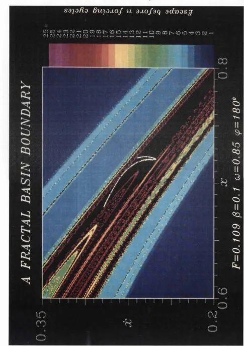
in the case of equation (1.2). With the appropriate change in the system parameters the inset and outset cross or tangle more; this leads to an increase in the width of the fractal boundary and an erosion of the basin of attraction of the stable spiral S1. The erosion of the basin of attraction of S1 occurs as the so called tongues, which are folds in the inset, are constrained to cross the outset thus distorting the shape of the basin of attraction further. This is illustrated in figure 1.3c. While a homoclinic tangency of a boundary saddle does not effect the local stability of the stable solution, which is governed by the local mapping eigenvalues, it is clearly an important event. For an engineer this may be as important as the final loss of stability of the stable solution. In a real life situation the marine vessel would never be allowed to settle down to some perfectly periodic motions for long. The period and amplitude of the forcing term would vary. Thus typical behaviour would be of a transient type decaying to a periodic stable solution. If the basin of attraction has been eroded by the homoclinic global bifurcation event, then the range of initial conditions which will lead to the stable periodic motion is reduced, effectively increasing the possibility of capsize. [16] has also shown that boundary explosions are intimately related to heteroclinic bifurcation events. Boundary explosions are events in which there is a sudden decrease in the size of the basin of attraction. Any change in the size of the basin of attraction of the stable solutions is of vital importance to engineers in a safety specification of the marine structure.
these algorithm is twofold: firstly for completeness and secondly because they represent an important foundation and background to all the work in this thesis. This section is mainly concerned with the Poincare phase space which is the Poincar6 section of a differential system. However as the Poincar6 map is an iterative map all the subsequent discussion, in this section, is directly applicable to other iterative maps, such as the Henon map of chapters 3 and 5. From now on in this thesis, the term Poincar6 phase space will be just phase space. As interest is primarily in mappings and not flows the distinction need no longer be maintained.
1.2.1 Global summaries of phase space.
Here the idea is to produce a diagram similar to figure 1.1 but for the Poincare section of mapping (1.2). This diagram is to describe all possible motions of the dynamic system while the parameters are constant. There are four methods available,
Grid o f starts method, Simple cell mapping, Generalised cell mapping and
Interpolated cell mapping.
In both these figures the boundary is touching the chaotic solution. This indicates a boundary crisis [16] which destroys the chaotic attracting solution. This is global bifurcation event, in fact a heteroclinic tangency. In both these figures the well developed fractal boundary can clearly be viewed. This method is of particular use when investigating fractal boundaries.
Simple cell mapping, SCM, Hsu [26] is based on the discretization of the phase space into a collection of rectangular cells. The value of the Poincare map functions
Fj and F2 are evaluated in the centre of every cell and here the SCM value is set equal to it. The assumption then is that everywhere else in the cell the SCM value is the same constant value as the centre of the cell. Thus SCM the replaces the Poincare map as the description of the motions in the phase space. Mathematically, the following descretised representation of the Poincare map defines the SCM,
S i( a ,b ) = F l(xi,y i)
S2(a ,b ) = F2(xl,y l)
x = I N T
yi = INT
\k j
where S} and S2 are the values of the SCM functions which approximate the
Fj and F2 Poincare map functions. A point (a,b) represents any point in phase space.
grid o f starts based on Poincar6 map; however it is an order of magnitude faster. In chapter 3, figure 3.7c is an example of a catchment basin described by the SCM method.
Interpolated cell mapping, ICM, Tongue [56] is based on a similar
discretization of the phase space into a collection of rectangular cells. Again the value of the Poincare map functions F1 and F2 are evaluated in the centre of every cell and here the ICM value is set equal to it. However the value of the ICM is not held constant across the cell as with the SCM. The actual value of the ICM at points not in the centre of a cell is bi-linearly interpolated from the values of the ICM in the centre of adjacent cells. This provides a continuity in the value of the ICM that SCM does not possess; thus is a much better approximation to the Poincare map. The computational overheads for the interpolation are small compared with the increase in accuracy. Thus the ICM replaces the Poincare map as the description of the motions in the phase space. Effectively the grid o f starts method can be reformulated using the approximation to the Poincare map the ICM. Pictures of basins of attraction and coloured transient time diagrams can be drawn. ICM represents considerable computational saving over the conventional grid o f starts
methods while being much more accurate than the SCM method.
probabilities. Pictures of basins of attraction and coloured transient time diagrams can be drawn. GCM is an improvement on SCM but is computational more expensive and more complex to implement. However it is still an order of magnitude faster than the grid o f starts method.
1.2.2 Problems of locating unstable solutions
While the methods in section 1.2.1 have great success in locating stable attracting solutions, unstable solutions such as saddles present a different problem altogether. The first approach is an off-shoot of the local bifurcation path following routines of chapter 4. The second in a method based on the invariant manifolds and a preliminary algorithm is sketched by Grebogi et al. [17].
Unstable solutions and stable solutions have the property that they are both fixed points in the Poincard map. By defining the return map or residual map as follows from the Poincare map (1.2),
G , = X i - j c , . i
G y = y , - y , . < 0 .3)
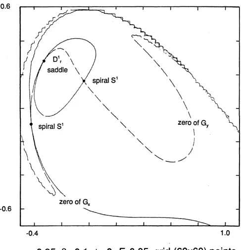
Consider 6figure 1.6: this is a diagram plotting the zero contours of the functions Gx
and Gy for the escape equation. Where these zero contours cross there must be a zero for equation (1.3) and a stable or unstable solution to (1.2). These contours are evaluated by suppling a grid of values of the functions Gx and Gy to a NAG [43] contour plotting routine which employs a bi-cubic spline interpolation to plot the zero contour lines. This is a useful technique as it indicates graphically where the zeros to equation (1.3) are in phase space. Figure 1.6 indicates there are three fundamental solutions. The two zero contours run very close to each other along the inset to the D1 saddle. This inset is described in section 1.1 as the boundary between the stable solution(s) S1 and the attractor an infinity. This figure indicates the problems a zero finding procedure would have if initiated in the region of the inset of the D1 hill top saddle in the escape equation (1.1). The position of the D 1 hill top
subharmonic saddles are generally heteroclinically tangled with the inset of the D1
hill top saddle. A consequence of this heteroclinic tangle is that these subharmonic saddles must lie on the inset to the D1 saddle. However this fact reduces the region of phase space in which a zero search need be performed. Grebogi et al. [17] uses this property to develop a simple algorithm for the location of higher periodic saddle cycles. This method could be extended and automated by describing the inset manifold by the algorithm INVAR in chapter 3. Then the algebraic set (1.3) are solved now the solution procedure is constrained to always remain on the inset described by INVAR. Further research into this method is required.
1.2.3 Invariant manifolds, local and global bifurcations.
Automotive production of invariant manifolds of saddle cycles is fully discussed in chapter 3. The work of Thompson [54] and Ling [33] are discussed and compared with the presented algorithm.
Local solution paths and local bifurcation paths in parameter/phase space are fully discussed in chapter 4. The work of Doedel [10], Holodniok et al. [24] and Kaas-peterson [29] are reviewed and compared with the presented algorithm.
Homoclinic and heteroclinic manifold tangency paths in parameter space are fully discussed in chapter 5. The work of Guckenheimer et al. [18], Hayashi et al.
[20], Holmes et al. [23], Kawakami [30], Yamaguchi et al. [62-63] are reviewed and compared with the presented algorithm.
1.2.4 Summary
cannot be just pulled out of the blue. Some knowledge of the system under analysis is a prerequisite for the use of such complex algorithms. This is a reminder that computation algorithms, for all their many subtleties, are not meant to replace understanding but to aid understanding. Thus, when in chapters 3, 4 and 5 respectively the algorithms for manifold production, local bifurcation path following and global bifurcation path following are discussed, the computational tools in sections 1.2 are assumed to be used to provide the background investigation required for the dynamic system under observation.
1.3 Review of thesis
ESCAPE FROM A POTENTIAL WELL
x + p x + x - x 2= F s i n c o t
VO
...
F
R
A
C
T
A
L
B
A
S
I
N
f i g u r e 1 . 4
s a p /i o
6uxojiof u axofaq adr>asg
+
FIGURE
1.5
s a ' i o f x o B u x o j c o f u a j t o f a q a d i o a s g
fr
CV2 C \2 C \2 O J CV] C \2 C \2 * -h ▼—i *— i »— \ *—.< «—< — « — * _ <
=
0
.
1
0
9
(
3
=
0
.
1
co
=
0
.
8
5
c
p
=
1
8
F igure 1.6
0 .6
-
0.6
saddle \
\
spiral S
zero of G
T spiral S 1
zero of G
2 Manifold tangency criteria.
It is clear that routines such as Kaas-Peterson’s PATH [29] and Doedel’s AUTO [10] have had considerable success in tackling the problems surrounding the description of local solution paths and local bifurcation loci. The ideology of these routines is to define a set of functions which, while varying across the parameter/phase space of the particular dynamic system involved, are constant at the local solution points and/or the local bifurcation points. The locus of local solutions or local bifurcations in parameter/phase space represents the solutions of the resultant fixed point problems. The specifics of local solution and bifurcation path following shall be discussed later (chapter 4.0). Thus as a technique the homoclinic/heteroclinic bifurcation path following algorithm, henceforth named MTA ( Manifold Tangency Algorithm ), follows on ideologically from its progenitors PATH and AUTO. MTA express its historical context by the introduction of another allegorical set of functions. These functions will constitute the manifold tangency criteria. This is at present loosely defined as a function which has a fixed point at tangency of the manifolds concerned. The general problem of the tangency of two manifolds in R m
phase space can be viewed as an extention of the problems in two dimensional phase space. Mostly this chapter will deal with this low dimensional analogue but the section 2.4.4 will draw out the extensions to higher dimensional systems.
2.1 Use of Fractal information.
the competing attracting basins which has become fractal. Generally not an easy task, Grebogi [17] describes a straight forward manual method which utilises information about the invariant manifolds, that is the stable and unstable manifolds of the boundary saddle cy cle. This is not, computationally, a useful basis for an automotive process as it requires sensitive tuning by the researcher and a knowledge of the current phase space under examination.
However there is one location where the boundary is known or can be found with greater ease. That is at the saddle point (a directly unstable point). The boundary locus of the competing basins of attraction is the closure of the inset of some boundary saddle, directly unstable point Stewart [48]. In the case of Thompson’s Escape equation [51-54] the boundary saddle is the D1 hill top saddle, (see examples is chapters 4 and 5) One of the outset eigenvectors of this saddle will always cross any fractal boundary. This is an implicit property of a fractal boundary that results from a homoclinic tangency bifurcation.
Consider the numerical scenario, for some two dimensional iterative map A, in which some short line vector L is chosen to be coincident with the linear approximation (local to the saddle point) of the outset. A discrete set of points Pq lying on L are chosen as initial conditions for the dynamic system under observation. This discrete set Eo contains points equispaced along the line vector L- Set £o maps to its image P x
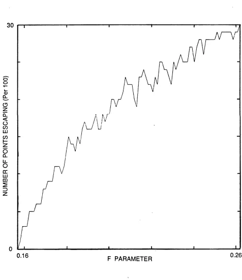
^.coincident with an outset eigenvectors and the observation of the images of JLunder the system mapping equations A can be thought of as a basis for a fractal formulation of a manifold tangency criterion. Consider the final destinations of the points in set £o in the above scenario. These can provide a measure of how far past tangency ( that is in a post tangency regime ) the dynamic system is at current parameter settings. Records of final destination will give an estimate of the thickness of the fractal boundary at the saddle point. The units of this thickness would in proportion to the number of points in the initial set Pq and the length of the line vector L- It could also provide, with a large number of points in the initial set£o, information about the density of the fractal boundary. This would be achieved by simply dividing the width of the fractal boundary, at the saddle, by the number of points with divergent final states.
The advantages of this idea are that the location of the saddle and eigenvectors is a local path following procedure and therefore straight forward, fig u re 2.0 represents some results from this method. Work on this method has shown certain deficiencies. Results produced under conditions mentioned below speak with an equivocacy which calls into question the algorithm value as an automotive process. The complications are (a) As is suggested by figure 2.0, the algorithm of section 2.1 provides no information
on the pre-tangency side. Reflect on an inset and outset, of a directly unstable saddle cycle, that are under conditions where there will be an imminent tangency under small perturbation of system parameters but are not at present at tangency.
The algorithm of considering the final destination of E& would result in all the images of points in Ex> mapping to the same attraction basin. Thus no fractal information can be provided before the fractal is formed. This lack of information would hamper any zero finding algorithm designed to locate where the all the starts £o just map to the same solution. An unconventional zero finding algorithm would need to be employed. As prediction of tangency is the final objective, this method would provide a highly ill-conditioned scenerio at tangency.
(b) When the phase space is simple, having only one solution point on either side of the boundary, the inset, and this solution being a fundamental or low order subharmonic solution, the suggested routine can discern on which side of the boundary the solution is. However in a more complex phase space where there are many coexisting high-order solutions, perhaps including chaotic solutions, it becomes very difficult to decide on which side of a probably complex tangled boundary the final attracting states of the points in the /2th image of Eo lie. (as
n oo)
2.2 Invariant manifold and point-wise comparisons.
The strength of the method discussed in section 2.1 is that finding and path following the saddle is a well documented process (AUTO [10] and PATH [29]) and reliable as an automotive procedure. By using a saddle’s eigenvectors the invariant manifolds, that is the stable and unstable manifold, can be extrapolated. Then considering the distance between the two manifold involved in the tangency, some distance-related function can be conjectured which has a fixed point at tangency. By adopting some formulation based on the geometric properties of tangency the one formulation is valid for many types of homoclinic and heteroclinic bifurcation events. The automotive production of the invariant sets is described in chapter 3. The algorithm INVAR produces a discretised set of points as an approximation to the continuous invariant set.
An initial algorithm could be to compare the distance of all the points on one manifold to all the points on the second manifold. Formally,
indicating the minimum distance between the points which describe the two
manifolds. However this procedure presents three main difficulties.
(a) Only information on the pre-tangency side would be obtained. Post-tangency distance between the two manifolds is always theoretically zero.
Sl(i) = {xl( i \ y l(i):i = h N l; i e Z }
s
2
(j)
= {x2(j),y2(j):j = 1 ,N2;j e Z}Anio = MIN (S,(i) - S2(j))2 for all i j
(b) For homoclinic problems the saddle itself would always represent an intersection of manifolds and would thus be a zero point in any distance function which would prejudice Dmin forcing its value to be zero.
(c) To increase the accuracy of the manifolds the number of points on the manifold must be increased (this is discussed in greater depth in chapter 3). As the numbers of points on each manifold increases the number of point-wise distance comparisons increases with its square. The procedure quickly becomes computationally expensive.
Consider the improvement to the above algorithm with the introduction of some gradient constraint. If distances between points of equal or nearly equal gradients are computed, and only these distances, this would answer all three problems.
Sj(0 = I, :i = e ZJ
S2U) = \ x2<j),y2< J ) ^ h -i = X' N* i e z ]
Minimise
{(*,(/) - x 2( j ) f +
Subject to
-e < arctan
dyi - arctan <E
manifold 1
manifold2
for all i , j
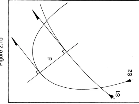
some curve line AL in the plane. Clearly the line AB can only represent a local minimum distance if the line AB if also perpendicular to curve AL. In this eventuality the gradients at A on AL and at B on BL must be coincident. Equality of gradients is a necessary condition but not sufficient for the minimum distance between two curved lines. This tangency condition is not sufficient because many points C and D on adjacent curves AL and BL may be of equal gradients but the the normal to curve AL at C and the normal to curve BL at D will not in general be coincident. In a post tangency situation where curves cross, the minimum distance is zero but the gradients cannot be equal. This last property is of real use as only under the tangency condition would intersecting curves have equal gradients and zero minimum distance. Consider *figure 2.1 : by imposing an equality of gradient constraint it yields useful information about the post tangency situation. Saddle points and intersection points can no longer be consider minima as they will not have equal gradients. The number of points with nearly equal gradient is relatively small and the time require to evaluate the gradients is of order n,
where n is the total number of points. This represents a computational saving as the number of points n increases.
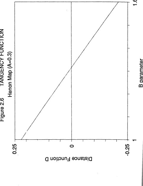
2Figure 2.2 represents some results of this pointwise comparison and gradient constraint method for pre and post tangency, equation (2.0). This is a graph of the constrained minimum distance evaluated by point-wise comparisons as a parameter B is varied for the Henon map, parameter A being constant at 0.3:
1.Figure 2.1: Expresses ideas of gradiant constraint minimisation of descrete point portraits of the invariant manifolds. Idealised definition of distance d in both pre-tangency and post-tangency situations.
x.+i=A-xl~By.,
y , * ,= x , .
However figure 2.2 shows substantial levels of noise on this graph. This would make any minimisation procedure designed to locate the tangency point by varying the parameter B almost impossible. The reasons for this noise are shown in !figure 2.3. The manifolds are only approximated by a set of points. As parameter B varies the position of the points along the manifolds may not be constant while the manifolds themselves may not vary much. This in itself is enough to produce high degrees of unreliability in the final constrained minimum distance as it is a result of these point-wise comparisons.
2.3 Cubic spline interpolation and constrained minimisation.
The problems of the last method in section 2.2 all result from the discretised form of the manifolds which algorithm INVAR produces. Consider the effect of handing the discretised set from INVAR to some multi-valued cubic spline interpolation based algorithm. McConalogue’s method [35] defines some new parametric variable S which is geometrically represents the arc-length distance along the manifolds. Consider a set of points I which approximates some invariant manifold.
( p c ,y ) e l
The coordinates of any point on the invariant manifold are expressed, parametrically, as two independant functions. This allows variables x and y to be intepolated in a straight forward manner by a conventional one dimensional cubic spline. The possibility of the manifold being multi-valued in x ory is no longer a problem. The above formulation would result in a continuous numerical function which is piecewise cubic and a much better approximation to the invariant manifolds. It generates a curve invariant under rotation but not under scaling: hence elements of the basis vectors should be equally scaled. Based on a now continuous set of curves, a real constraint minimisation routine can be used. This is formally express by the following:
D = Min {d (5 1,52)},
5152
d(S 1,52) = (x,(51)- x 2( S 2 ) f + (yx(S1) - >2(S2))2, (2.1) J J a y .(S l)l J3y2(5 2 )1 1
-- e < i arctan\ -r - ---- f - arctani ■ ■ ■ — f r < e.
I laxi(Sl)J [dx2(S2)\)
SI and S2 are arc-length variables. Work based on this formulation has indicated three main deficiencies.
(a) If the nonlinear constraint is too strictly enforced i.e. e is very small, then unless the initial guess solution is very near to the actual solution point even the best numerical routines for constraint minimisation find real difficulties in obtaining any solution.
points at which the manifolds intersect would still have nearly equal gradient. This would prove to be a zero for the formulation in equation 2.1 unless e is very small.
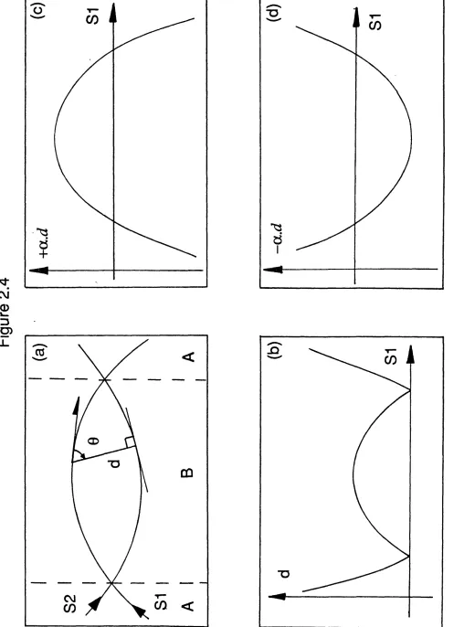
(c) In a post tangency regime the region B in figure 2.4a is a local maximum. Since the formulation 2.1 is a minimisation process it will inevitably lead to a solution which is coincident with the nonlinear constraint boundary. In effect the two inequality constraints will be satisfied one as an equality the other an inequality. This ambiguity in the solution will produce some unpredictability similar to the noise in figure 2.2, though not as marked.
The consequences of (a) and (b) are that the formulation has to be fine tuned in the value of the constraint e and also a good initial guess for the constrained minimum must be provided. This effect added to that of (c) seriously limits this formulation’s use as an effective procedure.
2.4 Maxi-minimisation and signing.
Consider also the post-tangency side of the parameter space. As one approaches tangency from this side the local maximum is reducing in size and thus becomes more difficult to locate. This is the situations of most interest as finally the aim is to locate the tangency bifurcation.
2.4.1 Tangency formulation.
pre-tangency:
post tangency:
tangency:
D~= Min {d (5 1,52)},
5152
D +- Max{±cc- Min{d(51,52)}1
51 52 J
a e B ,B = {-1 ,1 }
d(SU S2) = V(*i (S1) - x2(S 2))2 + (yi(51) - y 2(S 2))2,
D ~ = D+= 0 (2.2)
2.4.2 Signing.
fig u re 2.4a explains graphically the definition of the signing variable a . For this post tangency situation one can observe that on either side of an intersection point the actual sign of the angle 0 and hence a changes. The value of this property becomes apparent when one considers figure 2.4b. This figure is a plot of the way the minimized distance d(Sl,S2), with respect to 52, varies with SI for the situation of manifolds appearing in figure 2.4a. The problems with figure 2.4b as it stands are two fold.
(a) Around the crossing points the value of the minimized distance function reduces to zero. Due to nature of this unsigned distance function it is non-convex around this point. This leads to convergence difficulties of any maximisation or minimisation routine.
(b) Convergence to the maximum is difficult near to tangency on the post-tangency side.
A and positive in region B a negatively signed a must be used to ensure figure 2.4b becomes 2.4c. And again D+ can be evaluated. Here lies the problem: though the sign of angle 0 is known its correspondence to regions A or B is unknown as these regions are unknown until the final solution of D+. Thus, theoretically, both expressions with ± a must be evaluated. The expression corresponding to figure 2.4c will result in D+and the expression corresponding to figure 2.4d will diverge to some non-local solution.
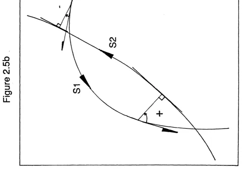
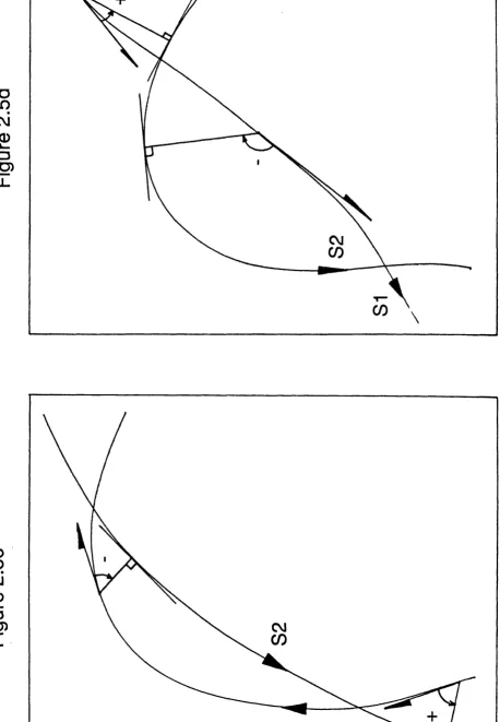
To be more precise about the nature of the signing process consider figure 2.5. Figures 2.5a and 2.5b show that the direction in which the arc-length variable S 1 is measured effects the angle 0 and hence a. However 2.5c shows that the direction in which S2 is measured has no effect on a. Figure 2.5d is a special case of figure 2.5b being rotationally transformed by n and the direction in which variable S2 is measured has no effect on signing.
While the manifolds many change in size and shape relative to one another as the control parameters are varied the topological signature of the manifolds at tangency will not change without the influence of some other global bifurcation event. The topological signature is the schematic shape of the manifolds which is not effected by any continuous distortions of the manifolds. Consequently often only one D+ will have to be evaluated as figure 2.5a and 2.5b do not have similar topological signatures in terms of the definition of their basis vectors.
observation. If D+ equals D' but is not equal to zero then the value of D' is a pre-tangency value for the tangency formulation. If the values D+ and D' are different then D' will be zero, this expression having found one of the intersection points. The value of the tangency formulation is then -D+ which is in a post-tangency situation. The negative sign indicates this distinction. Tangency itself is formulated in expression 2.2.
2.4.3 Angles.
Consider the following expressions for 0
The above formulation is a simple vector algebra expression for the angle between two vectors. The vector j is the unit base vector in the y cartesian direction.
.j a*i(si) ay.csn'
- 3S1 ’ 351 ,b = ( x , ( S1) - x 2(52),y,(51) - y2(S 2))
0, = arcsin (2.3.1)
0, = arcsin (2.3.2)
computationally. The main problem is the nature of the ARCCOS function as defined in most high-level programming languages such as Fortran 77, Pascal, C etc.. As an algebraic function ARCCOS is multi-valued but is defined as a single valued function in these programming languages. In Fortran 77 it’s range of values from +1 to -1 produces values of the ARCCOS function from 0 radians to n radians. This unsigned angle is of little use for the problem in hand. The above formulation fares a little better as even though ARCSIN is defined as a single valued function it includes some element of sign. The range of values from +1 to -1 produces values of the ARCSIN function from n/2 to -n/2. However angles greater than n/2 or less that -71/2 cannot be formally expressed by such a single valued function. This of course creates a problem for the last equation 2.3.3 as values of 0! and 02 from equations 2.3.1 and 2.3.2 are not always correct. To solve this problem a logic table was set up as follows for 0j and 02. This table effectively checks in which trigonometric quadrant the vector a lies and modifies the sign and perhaps the magnitude of 0!.
A A
a.i > 0 a.i < 0
a . j > 0 e, 7T-0!
a . j < 0 e, - 7 t- 0 j
*
b_.i > 0 b.i < 0
b j > 0
C
D n - 0 2
b j < 0 02 —K — 0 2
Thus by using equation 2.3 and the above logic tables all ambiguities caused be the representation of ARCSIN in the programming languages can be overcome.
2.4.4 m-dimensional formulation
The formulation of the manifold tangency criterion as given in section 2.4.1 remains much the same, save the distance function which is extended to an m-dimensional state space.
d (S 1,5 2) = V {(*t(S 1) - x2(S 2 ) f + (y,(51) - y2(S 2))2 + (2,(51) - z2(S 2))2 + ....}
Interest arises in the definition of a . Clearly the formulation in section 2.4.3 needs extension and modification. Tangent vector & and the vector fr are extended in the general problem to the following.
5.. /p i\ / r i \ N
vector £Xfc. The problem is to define an orthonormal basis in D such that an equivalent i j can be defined. £ is a vector orthogonal to a and a *b_ is thus orthogonal to a and in the plane D.
* _ £
*
\c\
3 I £ I
i and /d e fin e the orthonormal basis in D. Thus equations 2.3.1, 2.3.2 and 2.3.3 in section 2.4.3 can be redefined
0, = a r c s i n \ f ^ \ = 0
U f l l J
02 = a r , m |—
0 = - 6 2
The logic table in section 2.4.3 remains the same save b_.i is replace by b_.e
and b_.j by b_.f.
b .e > 0 b .e < 0
b . f > 0 02 7 t- 0 2
The above formulation extends the ideas in section 2.4 to higher dimensional state spaces.
2.5 Summary
N
U
M
B
E
R
O
F
P
O
IN
T
S
E
S
C
A
P
IN
G
(P
er
10
0)
Figure 2.0
30
0
0.26 0.16
F
ig
ur
e
2.
1a
F
ig
ur
e
2
.1
b
CM
F
ig
ur
e
2
.2
H
en
on
M
ap
(A=0.3)
C\J CVJ
o
• ■
o
o
P Sp|OJ!UB|/\J U00M109 0OUB1S1Q
B
p
a
ra
m
e
te
.Q CO
c\i
O )
U
CO CVJ
0) 1 _ 3
05
Fi
gu
re
2
.4
<D
F
ig
ur
e
2.
5a
F
ig
ur
e
2
.5
F
ig
ur
e
2.
5c
F
ig
ur
e
2
.5
d
CM
3 Production of Computational Portraits of Bounded Invariant Manifolds
In dynamics, global bifurcation events (Thompson and Stewart [54]) are of increasing interest because of their effect on ensembles of trajectories. Events such as heteroclinic and homoclinic tangencies can produce profound effects on the nature of the basin boundaries (Grebogi et al. [17]). Catastrophic bifurcations of chaotic attractors (Stewart [49]) while being important events are still difficult to systematically predict. Knowledge of the invariant manifolds of relevant saddle (hyperbolic) cycles is necessary as they are intimately involved in these events. For an engineer information about the final instability of an attracting solution and quantitative changes in the regions of attraction are vital in any safety specification. The ideas presented in this chapter represent an automation procedure for systematically describing these outstructures, that is these stable and unstable manifolds. The general problem of describing an m dimensional saddle ( m eigenvectors ) of period n in R m phase space can be viewed as an extension of the problem of describing a two dimensional saddle of period one in a two dimensional Poincarg section of phase space. (Consider the Poincard m ap/for forced oscillations. A period 1 saddlep corresponds to a periodic orbit of period T for the flow such that p -f(p ). A period n saddle corresponds to a periodic orbit of period nT such that p=fo(p) and p * f m(p) for 1 < m < n-1 where
k(p)=£&P)Y* etc- ) Mostly this chapter will deal with this low dimensional analogue of the generalised problem, though sections 3.1 and 3.6 will draw out the extensions to higher dimensional systems.
3.1 Location of the saddle
Consider a periodically driven differential oscillator
where 2 in as n-tuple of state variables, p is a vector function of period T and t is the independent variable. The Poincare section P can be defined as
P = { ( ± , t ) e R"*l:t = t0 + iT ,i e Z}.
From this periodic sampling of the solution space to (3.1) the Poincare map can be defined as the following vector equation,
& +i = ffe )- (3.2)
More generally, the hypersurface P need not be planar but must remain transverse to the flow. In general the time taken for an orbit in the flow to return to P will not remain constant. However a map of the form (3.2) can still be defined (Guckenheimer and Holmes [18])
A periodic cycle is now represented by a point or set o f points dependant on its periodicity. Thus a period one solution point is one at which consecutive iterates of (3.2) result in identical values. Consider the following equations,
£ & ) = £ +i - Xi , (3.3)
£ f e ) = f & ) - £ i > 3 /te )
dxj dxj
Jr =Jp I»
where I is the identity matrix. For a stability analysis of a solution point to (3.3) the eigenvalues of Jp must be found. The real eigenvalue problem can be thought of in terms of diagonalising Jr This requires a new vector basis to be found. When J? is transformed into this new basis it becomes diag( alv ..a,,) where ^ to an are the eigenvalues o f / p. The set containing all the eigenvectors is this new vector basis. Thus for a dynamic system the eigenvalues represent local independent scaling of the map along these vectors. For a saddle solution the eigenvectors are the locally linear approximations to the inset and outset.
Complex eigenvalues and eigenvectors can be handled by using complex variables for the eigenproblem: however the zero finding procedure must retain real variables. This effectively increasing the dimension of the Poincare section of phase space being considered. Degenerate cases where the eigenvalues repeat or their absolute values are equal to 1 must be dealt with as special cases. For higher dimensional systems the initial sets P0 ( section 3.2 ) must span the local stable and unstable eigenspaces.
3.2 Basic idea
in Q. maps to under a Poincare step with the qualifier that for the inset the inverse of the Poincard map must be used. This means simply integrating the system (3.1) in negative t.
The sets Pj represent a very close aproximation to the theoretical sets L;. Initial points £o of set P0on the inset/outset are extrapolated from the saddle by making use of the eigenvectors. The distance between these initial points and the saddle point must validate the linear assumptions while not being so small as to be obscured by the uncertainty about the numerical solution. The eigenvalues enable distinction between inset and outset to be made. The initial points £0 are mapped forwards/backwards to give on the outset/inset. Computationally the set P0can be expressed by dividing the line joining £0 and & into M points. By using the eigenvalues as an upper bound on the magnification, the number of points M required in P0to not need any insertion
of points in Pj can be computed .
3.3 Linked list
As set P0is mapped, the total length of the line element contained in its image sets Pi (i=l,n) will vary. Moreover the local scaling effects of different parts of the set may not be uniform. However knowledge about various subsets of P4and the way they will be scaled in P ^ can only be discovered after evaluating set P ^ (see section 3.8).
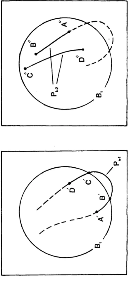
pointer array indicating the next data element to be looked at. Insertion/deletion in the data list requires only a change in two pointers not the re-ordering of the whole array. *Figure 3.1 explains this idea.
As Pj is mapped to p*. the distance Dj between consecutive points zi and Zj+i in PM is evaluated. If Dj is greater than Dmax then at least one point must be inserted between these two. This new point’s position can be predicted by taking the point that is linearly interpolated half-way between Zj and in Pj and mapping it into P ^ . This process is repeated until the inequality condition is satisfied. The interpolation is made in set Pj not in because it is the distance Djin Pi that is already bounded by D j ^ .
3.4 Bounds on manifold
Due to the infinite nature of the invariant set some bounds have to be placed on the set for the purpose of the numerical approximation. The first bound Bi to be considered is a geographic one, namely restricting interest to a certain region of Poincare section of phase space. This is often necessary purely for computational reasons arising, for example, from exponentially large phase space coordinates as the manifold stretches out towards infinity, this causing machine overflow. Consider 2figure 3.2 where set Pj is mapped partially across the bound in P ^ and back again in P ^ . Line element BC, subset of Pi is mapped ’out of bounds’ and hence points contained in this subset are lost, computationally. This, in turn, requires their deletion from the data list. Because many points may be deleted the locations of these now vacant cells in the data array are stored
1. Figure 3.1: Example of Linked list (a) standard Data list (b) and (c) insertion/deletion from list
in a stack data structure. The vacant cells can subsequently be used when insertion is required thus minimizing the space allocated for data. In figure 3.1(c) the INDEX of the DATA(2)=21. i.e. 2 would be stored in the stack. Another problem introduced by the sequence of events in figure 3.2 is the discontinuity in P ^ . Clearly the points must not be introduced between B" and C" in P*2by the method described in section 3.3, otherwise the image of the spurious straight line B ’C’ in P ^ will become part of P ^ . By introducing a negatively signed pointer in the pointer array at B ’ this allows the algorithm to remain aware of the discontinuity in the set Pj+2and not attempt to remedy it. The absolute value of the pointer array now indicates where the next data cell is in the list while the sign gives information about continuity.
procedure in 3.3 though the interpolated point now needs to be mapped n times forwards into the current set Pj. The only potential problem with bound B2is if part of the line element between % and ij+i of set Pj maps inside the bound B2 in P ^ while points and ij+i are still outside it. This bounded portion of the manifold would not be described. Due to the repetitive nature of homoclinic manifolds this may not be a great difficulty as all lines are described many times. However discretion should be exercised when considering the bound B2. It should include the saddle and all the complex topology of the Invariant manifold.
3.5 Algorithm
The program INVAR is the product of the following four sections. Section 3.5.1 is called once at the beginning. Section 3.5.2 creates set P0 for all insets and outsets. Sections 3.5.3 and 3.5.4 work together to describe the mapping of sets Pj to P^j and the insertion of points where required.
3.5.1 Locate saddle
1.0 Input initial guess for location of saddle.
2.0 Send to NAG [42] routine C05NCF to locate local zero 2.1 If NAG fails to converge, retry initial guess, goto 1.0
3.0 evaluate eigenvalues and eigenvectors of solution point by using NAG routine F02AGF.
3.1 If all eigenvalues are less than 1 then solution point is not a saddle point, retry initial guess, goto 1.0
4.0 END
3.5.2 Evaluate initial set P0
1.0 Extrapolate initial points £o in P0 from & and eigenvector 2.0 Map £o forwards/backward along the outset/inset to evaluate £i 3.0 Divide line joining £o and £ 1 into M points (set P0)
5.0 END
3.5.3 Map P0to Px
real array ZOLD(I J ) initially contains the points in set P0 and subsequently sets Pj. I indicates the INDEX position in the list while J indicates the coordinate ( J=1 is x, J=2 is y, J=3 is z, e tc .). Real array ZN EW (I J ) is similar to ZOLD but contains set P ^ . Integer array POINT(K) contains the I INDEX of the next ZOLD or ZNEW data in the list. Integer array STACK(L) contains the I INDEX of vacant location in ZOLD and ZNEW where points have been previously removed for exceeding bound B l. Integer STKP is the stack pointer indicating the top of the stack integers IP and IC are the previous and current I INDEX for ZOLD and ZNEW. Integer N, the current number of points in the list, is initially set to M. 1.0 Initialize integer variables
STK P=0: N=M 2.0 IP = 0 : IC=POINT(0)
3.0 from ZOLD(IC,J) evaluate ZNEW(IC,J), for differential equations this will require numerical integration ( classical Runge-Kutta)
4.0 if ZNEW(IC,J) outside bound B 1 then
4.1 reduce current number of points in the list N=N-1
4.2 if N is less than 2 then all of the current manifold has passed outside bound B 1 so return to section 3.5.2 to evaluate other parts of manifold. 4.3 record vacant location in ZOLD and ZNEW in the stack
STKP=STKP+1 : STACK(STKP)=IC
7.0 loop back to 3.0 for as long as there are point left in ZOLD to be mapped into ZNEW (that is points in Pt to be mapped to p ^ .)
8.0 if IC not equal zero then goto 3.0
9.0 END
3.5.4 Insertion of points, and output
Integer IC and IN are the current and next I INDEX of ZNEW. Real DMAX is the maximum allowable distance between consecutive points
1.0 IC=POINT(0): IN=AB S (POINT(IC))
2.0 if both points ZNEW(IC,J) and ZNEW(IN,J) are within bound B2 then 2.1 if distance between points ZNEW (ICJ) and ZNEW(IN,J) is greater
than DMAX and POINT(IC) is positive (that is no discontinuity) then insert point
2.1.1 if stack contain vacant cells (that is if STKP>0 ) use them 2.1.2 PT=STACK(STKP): STKP=STKP-1
if stack doesn’t contain vacant cells (that is if STKP=0 ) add on to the end of the list
2.1.3 M=M+1 : PT=M
set up pointers to direct list to new cell PT 2.1.4 POINT(IC)=PT : POINT(PT)=IN : IN=PT
If distance between ZOLD(IC,J) and ZOLD(IN,J) is less than DMAX then evaluate point ZOLD(PT,J) by interpolating
2.1.5 between points ZOLD(IC,J) and ZOLD(IN,J) and map this into ZNEW(PT,J) (section 3.3)
If distance between ZOLD(IC,J) and ZOLD(IN,J) is greater than DMAX then map points ZOLD(IC,J) and ZOLD(IN,J) back 2.1.6 until this distance conditions is satisfied. Then interpolate between
them and map the resultant point forwards in ZNEW(PT,J) (section 3.3)
4.0 output ZNEW(IC,J) and ZNEW(IN,J) to plotting routine. Draw line between them if they are within the plotting bounds.
5.0 reset ZOLD to ZNEW
ZOLD(IC, J)=ZNEW (IC, J) 6.0 move to next points
IC=IN : IN=AB S (POINT(IC))
7.0 loop back to 2.0 if IN is not equal to zero
8.0 if IN equals zero then end of list. Go back section 3.5.3 . ZOLD(IC,J)=ZNEW(IC,J)
goto section 3.5.3
9.0 END
3.6 Period w-order saddles
The ideas already presented can, with little modification, deal with these higher order solutions and their accompanying outstructures. Initially the period of sampling of the Poincare section is taken to be coincident with the period of the saddle and the
return map (3.3) defined on this new basis. In section 3.2 the initial points & are computed as before. Points & are n iterates of the period one Poincar6 map away from 2ofor a period /2-order direct saddle ( all positive real eigenvalues). Thus the initial set P0 contains a line element spanning n iterates. A period /2-order inverting saddle ( some negative real eigenvalues) is treated as a period /2-order direct saddle when defining the
3.7 Accuracy
The overall accuracy of the computational portrait of the manifold has a dual dependency on the local error of a point ^ in set P4 and the degree to which this is propagated in subsequent sets P ^ , PM etc.. Since the saddle and eigenvectors are evaluated extremely accurately (to within where e is machine precision) the first points £o are also very accurate. Moreover due to the hyperbolic nature of the saddle, locally there is always expansion along the outset and contraction along the inset in positive time t and vice versa in negative time t. When describing either outset or inset, locally, all trajectories are drawn towards the invariant set so initially the mapping procedure is a convergent one, onto the invariant manifold. Errors introduced in P0 are almost negligible. The main source of error is in the linear interpolation described in section 3.3. It can be shown that this local error is proportional to the curvature of the manifold and the square of the distance between the points. The degree to which this error is propagated is dependant on the divergence characteristics of the dynamic system.
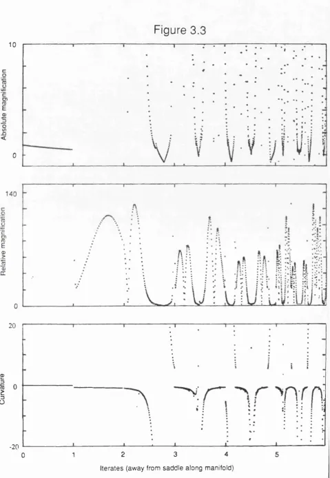
As a test case Thompson’s escape equation (3.4),[51-54] was used. This has a constant divergence of -p and thus for the map (3.2) a constant Jacobian determinant D (a cremona map). A region where there is magnification along the manifold, greater than D, requires a contraction perpendicular to the manifold. The degree of propagation of an error along the invariant manifold is inversely proportional to the magnification along the manifold. 3Figure 3.3 and 4figure 3.4 are records for the inset and outset of
the hill top saddle in the escape equation at parameter settings (P,co,cp,F) = (0.1,0.85, 0.0°, 0.075). The invariant manifold has a well developed homoclinic and perhaps heteroclinic structure. The curvature is evaluated by a finite difference expression. The relative magnification is the ratio of Dj in consecutive sets Pj and P ^ . The absolute magnification is the difference between Dj in Pj and P ^ normalised with respect to D j ^ . The horizontal axis represents the number of iterations away from the saddle, each integer block containing a set P*. The discontinuity at iteration equals 1 is not a property of the system dynamics but is due to the fact that consecutive sets Pj and P ^ will not in general have the same number of point elements. Thus is explained by a number of inserted points at the beginning of the list. Other discontinuities result from the fractured nature of set Pj (section 3.4). Both finite difference and linear magnification expressions are curvature and distance Dj dependant. That is at high curvature and magnification the accuracy of these approximate formulations comes into question. However only a qualitative feel for what is happening is required. The results produced showed an independence with variation in D * ^ confirming their underlying coherence.
all the local error terms it is difficult to make any specific generalization about global accuracy. However for systems with constant Jacobian determinant o f the map (3.2) there seem to be two distinct regions on the manifold. The production of regions that have low curvature and high magnification is a convergent process. The production of the other region, that of low magnification and high curvature, is eventually a divergent one (after a large number of iterations of the map away from the saddle).
3.8 Comparisons
Many researchers in the field of nonlinear dynamics use some kind of algorithm to evaluate the invariant sets. One of the simplest is to arrange a grid of start point sufficiently close to the saddle point and then observe the results of mapping them forwards and backwards. The local linear behaviour draws all the points towards the invariant set initially. Though this technique is straight forward it has many defects as an automotive process. The first draw back is the location of the saddle point which in general in not so easy to find without some process based on section 3.2. Second so to be within the locally linear behaviour of the saddle point its eigenvalues must be evaluated which again requires the saddle’s position. Thirdly the number of points in the initial grid that will be required to describe the manifold to even a few iterates will be orders of magnitude greater than the proposed algorithm. Finally it would be very difficult to automate any smooth curve plotting from the unordered resultant data. This is of more than just aesthetic value if one is to automate homoclinic and heteroclinic tangency locating routines one needs reliably ordered data.