Published online September 30, 2014 (http://www.sciencepublishinggroup.com/j/acis) doi: 10.11648/j.acis.20140205.11
ISSN: 2328-5583 (Print); ISSN: 2328-5591 (Online)
A novel artificial bee colony algorithm with an
overall-degradation strategy and its performance on the
benchmark functions of CEC 2014 special session
Bai Li
1, 2, 31School of Control Science and Engineering, Zhejiang University, Hangzhou, 310027, China
2School of Advanced Engineering, Beijing University of Aeronautics and Astronautics, Beijing, 100191, China 3Department of Chemical Engineering, National Tsing Hua University, Hsinchu, 30013, Taiwan
Email address:
[email protected]To cite this article:
Bai Li. A Novel Artificial Bee Colony Algorithm with an Overall-Degradation Strategy and Its Performance on the Benchmark Functions of CEC 2014 Special Session. Automation, Control and Intelligent Systems. Vol. 2, No. 5, 2014, pp. 71-80. doi: 10.11648/j.acis.20140205.11
Abstract:
The artificial bee colony (ABC) algorithm has been a well-known swarm intelligence algorithm, which assimilatesthe cooperating behavior of bees when seeking for nectar sources. Aiming to improve the conventional ABC algorithm, we focus on the re-initialization phase. In this paper, an overall-degradation-oriented artificial bee colony (OD-ABC) algorithm is proposed, pursuing to fight against premature convergence. This is achieved through re-initializing majority of the employed bees at one time, rather than generating at most one scout bee in each iteration. In this work, our OD-ABC algorithm is compared against the conventional ABC algorithms using 24 benchmark functions that origin from the CEC 2014’s competition on single objective real-parameter numerical optimization. The numerical results show that the OD-ABC algorithm is effective and thus can be employed to fight against premature convergence.
Keywords:
Artificial Bee Colony, Numerical Optimization, CEC 2014 Competition, Overall Degradation Strategy,Evolutionary Algorithm
1. Introduction
Investigations on evolutionary algorithms have been the focus of research for decades [1], which are designed in general for the derivation of optimal or near-optimal solutions of the objective functions [2].
The Artificial bee colony (ABC) is a swarm intelligence algorithm inspired by the foraging behavior of honey bees [3]. In this algorithm, the bee swarm mainly consists of three components, namely the employed bees, onlooker bees, and scout bees. In each cycle of iteration, the employed bees first carry out a global exploration. Those “qualified” employed bees then attract the onlooker bees to follow them. Due to the roulette selection strategy adopted in ABC, the relative qualification of each employed bee is related to its corresponding probability of being followed by onlooker bees. At the end of each iteration, “unqualified” employed bee will perish and then a randomly re-initialized scout bee
will take their places. It is worthwhile to notice that in the conventional ABC algorithm at most one scout bee can emerge in each iteration.
Regarding the modifications ever made for the conventional ABC, from the author’s viewpoint, the prevailing ways can be broadly classified into three categories. Methods in the first category usually adopt some strategies or theories from the outside world (e.g., see Refs. [21] and [22]). Those so-called hybridized algorithms that combine ABC with exterior techniques fall in this category as well. The methods in the second category mainly focus on making some small changes on the search equations of the conventional ABC (e.g., see Refs. [23-25]). Regarding the modifications in the third category, some changes in the algorithm’s framework should be carried out (e.g., see Refs. [8, 10, 17, 19, 26, 27]). Here in this work, our interest is focused on improving the conventional ABC algorithm using a strategy that falls in the third category.
We notice that the conventional re-initialization process in ABC is not competent to handle premature convergence, especially when a “super individual” in a swarm emerges, which denotes a discovered local optimal location that attracting nearly all the bees to search around. In our enhanced re-initialization procedure, we do not restrict it to generate only one scout bee at each time. We intend to accumulate such inefficiency convergence information and make the required changes all at once. We call this an overall-degradation strategy. In this work, we proposed a hybrid ABC algorithm combined with such overall-degradation strategy (namely the OD-ABC algorithm).
The remainder of this paper is organized as follows. In Section 2, we review the fundamental principle of the conventional ABC algorithm. In Section 3, we present the motivation that has inspired us to improve the conventional ABC algorithm. Then in Section 4, we describe our OD-ABC algorithm, followed by Section 5 where the numerical tests as well as experimental results are presented. Thereafter, we discuss our findings in Section 6, and finally, the concluding remarks are provided in the last section.
2. Conventional ABC algorithm
The conventional ABC algorithm employs three kinds of bees: scout bees searching for nectar sources randomly, employed bees associated with specific nectar sources, and onlooker bees following the guidance of employed bees. Typically, half of a bee colony would consist of the employed bees and the other half the onlooker bees [28].
At the very beginning, the scout bees are set out to randomly search for nectar sources. Thereafter, they are replaced by employed bees responsible for global exploration. During the global exploration procedure, those employed bees can share information (i.e., nectar source quality and the current location) with companions by means of “dancing”. Then the onlooker bees select the nectar sources that the employed bees have discovered to exploit. It is worth pointing out that relatively higher-quality nectar sources are more likely to be chosen by the onlooker bees to exploit (as a natural consequence of utilizing the roulette
selection strategy). If an employed bee finds no better nectar source than the one that it has previously discovered within a certain cycle, it turns into a scout bee again, which implies that its position will be randomly initialized in the search space.
A location of a nectar source represents a feasible solution to the problem, and the nectar quantity is reflected by the objective function value. Let 1 2
1
X ( , , , D)
D
X X X ×
= ⋯
represent a solution in the feasible solution space, fun( )⋅ be the objective function that needs to be minimized,
( , )
rand m n be a random number between m and n obeying the uniform distribution, and SN be the population size of a bee swarm. As aforementioned, the number of onlooker bees in a bee colony is
2
SN , equalling that of the employed bees.
At first, as many as 2
SN scout bees are randomly initialized in the feasible solution space. Equation (1) shows how the jth element of the ith scout bee’s location Xi is calculated:
{
}
{
}
min (0,1) ( max min),
1, 2,..., , 1, 2,..., , 2
j j j j
i
X X rand X X
SN
i j D
← + ⋅ −
∈ ∈ (1)
where min
j
X and max
j
X denote the lower and upper boundaries of this jth element, and D denotes the
dimension of a feasible solution. Thereafter, the SN2 scout
bees will become the employed bees and an iterated process begins from here.
In each cycle of iteration, an employed bee will share information with a randomly chosen companion and change one randomly chosen element of its location vector from j
i X
to *j i
X using the following equation:
{
}
{
}
*
( 1,1) ( ),
1, 2, , , 1, 2, , , . 2
j j j j
i i k i
X X rand X X
SN
k j D k i
← + − ⋅ −
∈ … ∈ … ≠
(2)
It is necessary to note that j and k are both randomly selected integers. When all the employed bees arrive at their
new nectar sources X*i i∈
{
1, 2,…,SN2}
, they evaluate thequality of these new nectars and then decide whether to stay at the new location or the previous one by means of a greedy selection strategy. Specifically, if the ith employed bee finds that *
(X )i (X )i
fun < fun , it will go to the new location
*
Xi , i.e., *
Xi ←Xi ; otherwise, it remains at the previous location Xi.
{
}
2 1
( ) , 1, 2, , ,
2
SN
j
fitness i SN
P i i
fitness j
=
= ∈
∑
…( )
( ) (3)
1
if (X ) 0 1 (X )
( ) .
1 (X ) if (X ) 0
i i i i fun fun fitness i fun fun ≥ + =
+ <
(4)
Each onlooker bee will search locally around an employed bee. For some ith onlooker bee, a comparison is made between a random number rand(0,1) and P j( ) . If
( ) (0,1)
P j ≥rand , this onlooker bee will search around the th
j employed bee; otherwise, a comparison between
(0,1)
rand and P j( +1) will be made. If even ( ) 2 SN P
happened to be smaller than rand(0,1), such a comparison process is repeated from the first employed bee’s P(1) again until a larger P j( ) is found. Then, the corresponding jth employed bee will be chosen. The following equation (i.e., Equation (5)) shows the location of the ith onlooker bee
(
1 1 1)
1
Y , , k , k, k , , D
i Xj Xj Yi Xj Xj D
− +
×
= … … that searches locally
around the selected jth employed bee.
{
}
{
}
( 1,1) ( ),
1, 2, , 2 , 1, 2, , , .
k k k k
i j m j
Y X rand X X
SN
m k D m j
← + − ⋅ −
∈ … ∈ … ≠
(5)
Note that in this equation m and k are randomly selected integers as well. When all the
2
SN onlooker bees have
determined their locations, a greedy selection strategy is implemented. This time, however, a comparison is made between fun(X )j and fun(Y )i ,
{
1, 2, ,}
2
SN
i∈ … . If
(Y )i
fun is smaller than fun(X )j , the jth employed bee will discard its current location Xj and fly to Yi , i.e., Xj ←Yi; otherwise, the jth employed bee remains at Xj. It is interesting to point out that every time the greedy selection is carried out, it involves one central employed bee. There is an index that is associated with each of the employed bees, namely trial , which memorizes inefficient search times that concerns each of the employed bees. Specifically,
( )
trial i records the number of times that the ithemployed bee has searched inefficiently. That is, trial i( ) is incremented by one each time when the condition
*
(X )i (X )i
fun ≥ fun or fun(Y )j ≥ fun(X )i is satisfied. At the beginning, each trial i( ) is set to zero. As the iteration goes on, when trial i( ) reaches a predefined threshold Limit, the
th
i employed bee will turn into a scout bee again.
3. Motivation
In this section, we elaborate on the reason why it is advisable to make some changes in the re-initialization phase of ABC [1].
At the end of each iteration, having just one scout bee at most to be generated during the re-initialization phase limits the capability of the algorithm to overcome premature convergence. As a matter of fact, it has been confirmed in some numerical experiments that directly discarding the scout bees will not necessarily deteriorate the convergence performance [29].
Particularly, when a “super individual” (i.e., a discovered local optimal location that attracting nearly all the bees to search around) emerges in a swarm, such re-initialization process is not efficient at all to overcome. Once an employed bee is re-initialized in one iteration, it is likely to be attracted back to the same local optimal location again since other companions are still gathering around that place.
The emergence of super individuals is one cause of premature convergence in swarm intelligence algorithms. Another chief cause may be that the search domain is too large, thus making the optimization process slow to converge. In such cases, re-initializating a majority (but not all) of bees in the colony will be a feasible way to improve the situation.
In the next section, we will introduce the OD-ABC algorithm in detail.
4. Overall-degradation ABC Algorithm
The OD-ABC is different from the conventional ABC algorithm in the re-initialization phase. Here, before a new iteration begins (i.e., at the end of each iteration), any trial i( ) that has exceeded Limit will be reset to Limit (rather than
0). Thereafter, average value of trial (i.e., 2 1
2
( )
SN
i trial i
SN
∑
= )is compared to αodr⋅Limit , where α ∈odr
( )
0,1 is a user-specified scalar. If α ⋅odr Limit is smaller than2 1
2
( )
SN
i trial i
SN
∑
= , the whole swarm is considered to be not working efficiently to a degree of αodr. Then, as many as(
)
round
2
odr SN
α ⋅ randomly selected employed bees will be re-initialized according to Equation (1). At the same time, their corresponding trial indices should be reset to zero. If
2 1
2
( )
SN
i trial i
SN
∑
= is smaller, the current iteration is terminated directly and a new iteration will begin.Algorithm 1. OD-ABC Algorithm
1. Set the population size SN, overall degradation rate αodr, and
maximum cycle number MCN; Set the invalid trial time counter
( ) 0
trial⋅ ← (
{
1, 2, ,}
) 2 SNi∈ … ;
2. Randomly initialize locations of SN2scout bees using Equation (1);
3. For iter=1 to MCN, do
4. For item=1 to SN2, do % the employed bee phase
5. Generate *
Xitem for the item-th employed bee to search according
to Equation (2);
6. If *
(Xitem) (Xitem)
fun <fun , then % implement the greedy selection
7. *
Xitem←Xitem, and set trial item( )←0;
8. Else
9. trial item( )←trial item( ) 1+ ; 10. If trial item( )>Limit, then 11. trial item( )←Limit
12. End if 13. End if 14. End for
15. For i=1 to SN2, do % prepare for the roulette selection
16. Calculate ( )P i using Equations (3) and (4); 17. End for
18. Set j=1; 19. Set item=0;
20. While item<SN2, do % implement the roulette selection
21. If ( )P j >rand(0,1), then % the onlooker bee phase
22. item←item+1;
23. Choose the thj employed bee to follow, and then generate
Yitem using Equation (5);
24. If fun(Yitem)<fun(X )j , then % implement the greedy
selection
25. Xj←Yitem, and set trial j( )←0;
26. Else
27. trial j( )←trial j( ) 1+ ; 28. If trial j( )>Limit, then 29. trial j( )←Limit
30. End if 31. End if 32. End if 33. j← +j 1; 34. If j>SN2, then 35. Set j←1; 36. End if 37. End while
38. If 2 1 2
( )
SN
odr i trial i Limit
SN
∑
= >α ⋅ , then % implement the overall degradation strategy39. Randomly re-initialize as many as round
(
α ⋅odr SN2)
employedbees’ locations according to Equation (1);
40. Set their corresponding scalars trial( )⋅ ←0;
41. End if
42. Memorize the best solution; 43. End for
44. Output the best solution;
Initialize food source using Eq. (1) Set trial= 0, iter= 0.
Start
iter= iter+1
iter>MCN?
Generate each of the employed bees using Eq. (6)
Is better position derived for i-th employed bee?
Set trial(i) = 0
Select employed bee for each onlooker to follow using Eqs. (3) and (4)
Is better position derived for j-th employed bee?
Let trial(j) = trial(j) + 1
Output best position
End Y N N Y N Y
Set trial(j) = 0 Let trial(i) = trial(i) + 1
Store best position in the current iteration
Generate each of the onlookers using Eq. (5) (choose j-th employed bee to follow)
Set such trial to Limit
Any trial exceeds Limit? Y
N
mean(trial)>
odrLimit? N
Y selected employed bees using Eq. (1);Re-initialize (100 odr )% randomly Set corresponding trial(·) = 0
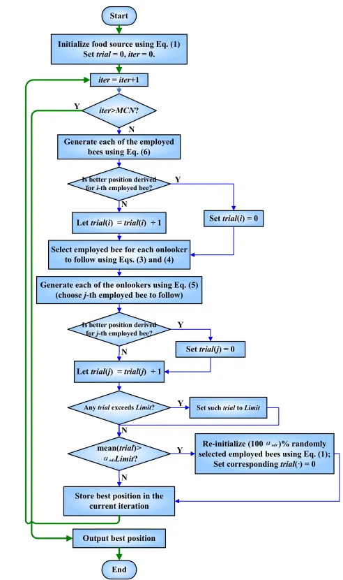
Fig 1. A flowchart of OD-ABC algorithm.
5. Experiments and Results
In order to see the performance of the OD-ABC algorithm in comparison with the conventional ABC algorithm, we systematically conducted a number of comprehensive simulation experiments (i.e., the first 24 benchmark functions for the competition of the CEC 2014 Special Session [30]). In all our computational experiments, the maximum number of cycles MCN was constantly set to 5000 and the swarm population (i.e., 2⋅SN ) was set to 40 for both algorithms involved. Each of the experiments was repeated for 30 times with different random seeds. The search range is constantly set to [ 100,100]− Dim
, where Dim=50 refers to the dimension of the benchmark problems in this work. All the simulations were carried out in a Matlab R2011b environment and executed on a Intel Core 2 Duo CPU with 2GB RAM running at 2.53 GHz under the Microsoft Windows XP operating system.
In the last columns of this table, we report the statistical significance level of the difference of the means of the results produced by the best and the second best algorithms (with respect to their final accuracies). Note that here “p value” reveals the chance if the null hypothesis (the differences between OD-ABC and ABC can form a normal distribution) is true. ‘+’ indicates the OD-ABC works better than ABC at a
0.10 level of significance by two-tailed test; ‘-’ indicates the ABC works better than OD-ABC at a same level of significance; while ‘.’ indicates the two algorithm show no difference in statistics.
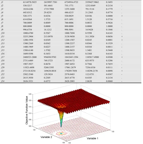
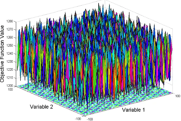
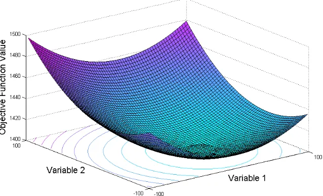
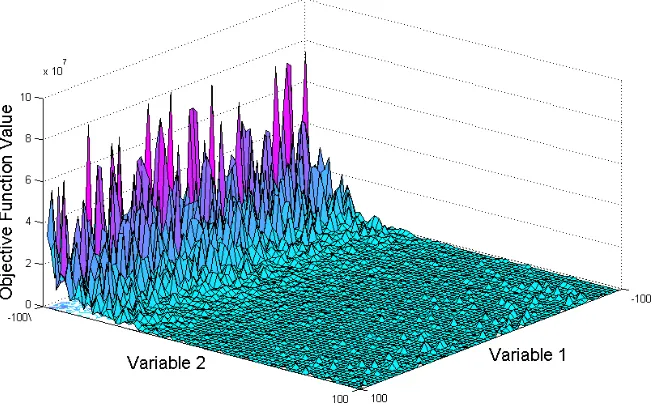
Three-dimensional visualization of a selected number of two-dimensional benchmark functions are illustrated in Figs. 2-10.
Table 1. Result comparisons of ABC and OD-ABC on 24 benchmark functions in CEC 2014’s competition.
Test Function ABC OD-ABC p-value Significance
Mean S.D. Mean S.D.
f1 6114570.5025 2419997.7581 6724954.4722 3359427.9062 0.3493 .
f2 530.5217 581.4641 755.1771 1232.0369 0.2134 .
f3 1818.6106 1719.7908 1355.3680 791.5116 0.1779 .
f4 445.8312 29.4235 446.6215 31.2563 0.8774 .
f5 520.1571 0.0236 520.0829 0.0186 0.0000 +
f6 614.8564 1.5735 615.1491 1.5120 0.5716 .
f7 700.0009 0.0049 700.0006 0.0032 0.9426 .
f8 800.0000 0.0000 800.0000 0.0000 1.0000 .
f9 996.6754 14.1212 990.5091 14.9428 0.1846 .
f10 1000.6780 0.5567 1000.7694 0.5598 0.6143 .
f11 3255.2904 213.0970 3138.9450 311.3926 0.0656 +
f12 1200.1958 0.0349 1200.1587 0.0245 0.0001 +
f13 1300.2369 0.0362 1300.2237 0.0366 0.1529 .
f14 1400.1969 0.0227 1400.2157 0.0184 0.0011 -
f15 1508.6140 1.5702 1508.9653 1.3481 0.5440 .
f16 1609.9398 0.3453 1610.0154 0.3368 0.6143 .
f17 2408523.2800 956030.9703 1841845.1394 1105817.4900 0.0300 +
f18 2731.6489 749.3723 2480.4172 633.9575 0.3286 .
f19 1907.3927 0.8670 1907.4452 0.7566 0.7655 .
f20 11923.4498 5260.5395 17061.2679 7256.6336 0.0111 -
f21 272118.8254 149638.8018 178289.7058 118298.2170 0.0098 +
f22 2502.2540 129.5824 2570.8483 112.8751 0.0387 -
f23 2615.3930 0.2305 2615.4770 0.4185 0.2134 .
f24 2626.3521 6.6572 2628.2003 2.0630 0.0060 -
Fig 3. 3-D visualization for 2-D benchmark function 9.
Fig 4. 3-D visualization for 2-D benchmark function 11.
Fig 6. 3-D visualization for 2-D benchmark function 17.
Fig 7. 3-D visualization for2-D benchmark function 21.
Fig 9. 3-D visualization for 2-D benchmark function 22.
Fig 10. 3-D visualization for 2-D benchmark function 24.
6. Discussion
According to the results listed in Table 1, we find that in most cases, the OD-ABC algorithm cannot outperform the conventional ABC algorithm with statistical significance. However, it is worthwhile to notice that the several benchmark functions that OD-ABC works better on (see Figs. 2-7) are far more complicated than the ones that ABC works better on (see Figs. 8-10). As in Figs. 2-7, there are in general a large number of local minimums around the global optimum, making it difficult to overcome premature convergence. In contrast, local minimums are not so close to the global optimums in the cases of benchmark functions 14, 22 and 24. All the mentioned above indicate that, the OD-ABC algorithm works well to handle the objective functions that are more challenging.
7. Conclusion
In this paper, we have proposed an OD-ABC algorithm, the main idea of which is to provide a more efficient re-initialization phase in the algorithm’s framework. The innovations and highlights of in this work can be summarized as follows.
Despite these highlights and innovations, we confess there is still room for improvement since OD-ABC becomes inefficient when tested on some unimodal and/or simple multimodal benchmarks. As a feasible suggestion, combining such overall-degradation strategy with other existing strategies may work (e.g., see Refs. [1, 7, 31]).
After all, we believe that the unique and promising idea behind our OD-ABC algorithm is worth pursuing further.
Acknowledgements
The author declares that there is no conflict of interests regarding the publication of this paper. This work was supported in part by the 6th National College Students’ Innovation & Entrepreneurial Training Program in China under Grant No. 201210006050.
References
[1] B. Li, R. Chiong and R. Zhang, Balancing Exploration and Exploitation: An Analysis of the Balance-Evolution Artificial Bee Colony Algorithm, unpublished.
[2] D. Dasgupta and Z. Michalewicz (Eds.). Evolutionary algorithms in engineering applications. Springer Berlin Heidelberg, 1997.
[3] D. Karaboga and B. Akay, A modified artificial bee colony (ABC) algorithm for constrained optimization problems,
Applied Soft Computing, Vol. 11, No. 3, pp. 3021-3031, 2011.
[4] D. Karaboga and B. Basturk, A powerful and efficient algorithm for numerical function optimization: artificial bee colony (ABC) algorithm, Journal of global optimization, Vol. 39, No. 3, pp. 459-471, 2007.
[5] B. Li, L. G. Gong and C. H. Zhao, Unmanned combat aerial vehicles path planning using a novel probability density model based on Artificial Bee Colony algorithm, In 2013 Fourth International Conference on Intelligent Control and Information Processing (ICICIP 2013), pp. 620-625, IEEE, 2013.
[6] H. Duan, S. Shao, B. Su and L. Zhang, New development thoughts on the bio-inspired intelligence based control for unmanned combat aerial vehicle, Science China Technological Sciences, Vol. 53, No. 8, pp. 2025-2031, 2010.
[7] B. Li, L. G. Gong and W. L. Yang, An improved Artificial Bee Colony algorithm based on balance-evolution strategy for unmanned combat aerial vehicle path planning, The Scientific World Journal, Vol. 2014, No. 23704, pp. 1-10, 2014.
[8] B. Li, L. G. Gong and Y. Yao, On the performance of internal feedback artificial bee colony algorithm (IF-ABC) for protein secondary structure prediction. In 2013 Sixth International Conference on Advanced Computational Intelligence (ICACI 2013), pp. 33-38, IEEE, 2013.
[9] H. Sun, H. Luş and R. Betti, Identification of structural models using a modified Artificial Bee Colony algorithm, Computers & Structures, Vol. 116, pp. 59-74, 2013.
[10] B. Li, Y. Li and L. G. Gong, Protein secondary structure optimization using an improved artificial bee colony algorithm based on AB off-lattice model, Engineering Applications of Artificial Intelligence, Vol. 27, pp. 70-79, 2014.
[11] R. J. Kuo, Y. D. Huang, C. C. Lin, Y. H. Wu and F. E. Zulvia, Automatic kernel clustering with bee colony optimization algorithm, Information Sciences, Vol. 283, pp. 107-122, 2014.
[12] B. Li, Research on WNN modeling for gold price forecasting
based on improved Artificial Bee Colony
algorithm, Computational intelligence and neuroscience, Vol. 2014, No. 270658, pp. 1-10, 2014.
[13] Q. K. Pan, M. Tasgetiren, P. N. Suganthan and T. J. Chua, A discrete artificial bee colony algorithm for the lot-streaming flow shop scheduling problem, Information sciences, Vol. 181, No. 12, pp. 2455-2468, 2011.
[14] J. Q. Li, Q. K.Pan and K. Z. Gao, Pareto-based discrete artificial bee colony algorithm for multi-objective flexible job shop scheduling problems, The International Journal of Advanced Manufacturing Technology, Vol. 55, pp. 1159-1169, 2011.
[15] L. Wang, G. Zhou, Y. Xu, S. Wang and M. Liu, An effective artificial bee colony algorithm for the flexible job-shop scheduling problem, The International Journal of Advanced Manufacturing Technology, Vol. 60, No. 4, pp. 303-315, 2012.
[16] M. F. Tasgetiren, Q. K. Pan, P. N. Suganthan and A. H. Chen, A discrete artificial bee colony algorithm for the total flowtime minimization in permutation flow shops, Information Sciences, Vol. 181, No. 16, pp. 3459-3475, 2011.
[17] B. Li, L. G. Gong and Y. Li, A Novel Artificial Bee Colony Algorithm Based on Internal-Feedback Strategy for Image Template Matching, The Scientific World Journal, Vol. 2014, No. 906861, pp. 1-14, 2014.
[18] C. Chidambaram and H. S. Lopes, An improved artificial bee colony algorithm for the object recognition problem in complex digital images using template matching, International Journal of Natural Computing Research, Vol. 1, No. 2, pp. 54-70, 2010.
[19] B. Li and Y. Yao, An edge-based optimization method for shape recognition using atomic potential function, Engineering Applications of Artificial Intelligence, Vol. 35, pp. 14-25, 2014.
[20] C. Xu and H. Duan, Artificial bee colony (ABC) optimized edge potential function (EPF) approach to target recognition for low-altitude aircraft, Pattern Recognition Letters, Vol. 31, No. 13, pp. 1759-1772, 2010.
[21] W. F. Gao, S. Y. Liu and L. L. Huang, A novel artificial bee colony algorithm with Powell's method, Applied Soft Computing, Vol. 13, No. 9, pp. 3763-3775, 2013.
[22] F. Kang, J. Li and Z. Ma, Rosenbrock artificial bee colony algorithm for accurate global optimization of numerical functions, Information Sciences, Vol. 181, No. 16, pp. 3508-3531, 2011.
[23] G. Zhu and S. Kwong, Gbest-guided artificial bee colony algorithm for numerical function optimization, Applied Mathematics and Computation, Vol. 217, No. 7, pp. 3166-3173, 2010.
[25] W. L. Xiang and M. Q. An, An efficient and robust artificial bee colony algorithm for numerical optimization, Computers & Operations Research, Vol. 40, No. 5, pp. 1256-1265, 2013.
[26] A. Alizadegan, B. Asady and M. Ahmadpour, Two modified versions of artificial bee colony algorithm, Applied Mathematics and Computation, Vol. 225, pp. 601-609, 2013.
[27] B. Li and Y. Li, Y, BE-ABC: hybrid artificial bee colony algorithm with balancing evolution strategy, In 2012 Third International Conference on Intelligent Control and Information Processing (ICICIP 2012), pp. 217-222, IEEE, 2012.
[28] B. Li, R. Chiong and L. G. Gong, Search-Evasion Path Planning for Submarines Using the Artificial Bee Colony Algorithm, In Proceedings of the IEEE Congress on Evolutionary Computation (CEC 2014), pp. 528-625, IEEE, 2014.
[29] D. Karaboga and B. Basturk, B, On the performance of artificial bee colony (ABC) algorithm, Applied soft computing, Vol. 8, No. 1, pp. 687-697, 2008.
[30] J. J. Liang, B. Y. Qu and P. N. Suganthan, Problem definitions and evaluation criteria for the CEC 2014 special session and competition on single objective real-parameter numerical optimization, Technical Report 201311, Computational Intelligence Laboratory, Zhengzhou University, Zhengzhou China and Technical Report, Nanyang Technological University, Singapore, 2013..