Simulation, Optimization & Control of Styrene Bulk Polymerization in a Tubular Reactor

Simulation, Optimization & Control of

Styrene Bulk Polymerization in a Tubular Reactor

Ghafoor Mohseni, Padideh; Shahrokhi, Mohammad*+ Chemical and Petroleum Engineering Department, Sharif University of Technology,

P.O. Box: 11365-9465 Tehran, I.R. IRAN

Abedini, Hossein

Iran Polymer and Petrochemical Institute, P.O. Box: 14965-115 Tehran, I.R. IRAN

ABSTRACT: In this paper, optimization and control of a tubular reactor for thermal bulk post-polymerization of styrene have been investigated. By using the reactor mathematical model, static and dynamic simulations are carried out. Based on an objective function including polymer conversion and polydispersity, reactor optimal temperature profile has been obtained. In the absence of model mismatch, desired product characteristic can also be obtained by applying the corresponding reactor wall or jacket temperature profile. To achieve this temperature trajectory, reactor jacket is divided into three zones and jacket inlet temperatures are used as manipulated variables. Effectiveness of the proposed approach has been demonstrated through computer simulation. Furthermore for a special case of model mismatch, a method has been proposed which results in a near optimal profile.

KEY WORDS:Dynamic simulation, Tubular reactor, Styrene bulk polymerization, Optimization, Control.

INTRODUCTION

Polystyrene is one of the major commodity thermo- plastics in the world. Continuous bulk styrene polymerization reactors are generally classified into two groups: the back mixed reactor and the Linear-Flow Reactor (LFR). Bulk styrene polymerization is always accompanied with a large heat generation and high viscosity. The choice of polymerization reactor depends on the desired polymer quality/quantity. Multiple reactor stages can be tailored in a number of ways to meet specific product needs. Most polystyrene licensors and/or

producers still stay with two or more reactors in series to maintain production flexibility [1-4]. Due to the advantages of tubular reactors, regarding simple design and low cost, it is desired to use this type of reactor in polymerization processes [2, 4-6]. Studies of various aspects of polymerization in tubular reactors have been reported in the literature. Using different models for the process, the parametric sensitivity, stability, optimization and control have been considered [7-12]. Many theoretical and experimental works have been done

*To whom correspondence should be addressed. +E-mail:[email protected]

to study the feasibility and operability of bulk polymerization in tubular reactors [7-9]. In all of these works, the tubular rector has been considered as a post polymerization reactor and both axial and radial variations have been taken into account and a two-dimensional steady state model for the reactor has been considered. A commercial process for polystyrene production has been proposed by Chen [8]. It is desired to obtain maximum monomer conversion and a polymer with minimum possible polydispersity. Costa et al. [10] used the two dimensional steady state model proposed by Chen [8] and based on an objective function, optimal reactor wall temperatures through a multi objective optimization method has been obtained.

In industry, usually a series of reactors of different or similar types are used in polymerization processes [13]. The configuration proposed by Chen [8] for producing polystyrene consists of a CSTR (for polymerization up to 75%) followed by a tubular reactor to achieve product with about 90% conversion and more. Based on cumulative moment method, dynamic simulation of a two-stage continuous bulk styrene polymerization process is investigated by Gharahni et al. [14]. Also temperature control of auto-refrigerated continuous stirred tank reactor and tubular reactor by PI controllers are carried out, simultaneously.

In this work, radical thermal bulk polymerization of styrene in a tubular reactor, served as post polymerization, has been studied. In this paper, based on the work of Chen [8], first the mathematical model for the reactor is presented. In most of previous works static simulation and optimization have been considered but no practical way for implementation of optimal temperature profile along the reactor length had been mentioned. In this contribution, three optimization policies have been defined to minimize the selected objective function. Results of these three optimization problems provide reactor, wall and jacket temperature profile for the reactor. By using the static model, feasibility of implementation of optimization results have been studied. A control strategy is proposed to keep the desired temperature profile along the reactor length and its effectiveness has been shown trough simulation. Finally a special case of model mismatch has been taken into account and a strategy is proposed for handling the model uncertainty.

MODELING

Based on mass and energy balances, the reactor mathematical model has been derived. It is assumed that static mixers are installed inside the reactor and therefore radial gradients of concentration, temperature and velocity are neglected. The flow pattern in the reactor is assumed to be plug flow [8]. Due to mixers effects, reactor model has less mathematical complexity and uniform residence times are obtained for the material inside the reactor (plug flow) and hence heterogeneity in the product is decreased. Furthermore, using of static mixers is an aid for effective heat removal from the reactor, which is crucial for highly exothermic reactions such as polymerization reactions.

By writing mass and energy balances, the following equations are obtained [8]:

m m z p V R t z ∂ω ∂ω ρ = −ρ −

∂ ∂ (1)

p p z p ₂

T T Q

c c V R H

t z R

∂ ∂

ρ = − ρ − ∆ +

∂ ∂ π (2)

i j w o o j j

Q=h (2 RL )(Tπ −T)=U (2 R L )(Tπ −T) (3)

j

j p, j j j p, j j,in j

dT

V c F c (T T ) Q

dt

ρ = − − (4)

The free-radical polymerization of styrene has already been extensively investigated in the literature. Therefore, rate constants and other kinetic parameters used in this work are those which are provided by other researchers [8, 15]. The kinetic mechanism considered here involves the following basic steps [15].

Thermal initiation:

i k

1

3M→2R• (5)

Propagation:

p k

r r 1

R M R

• •

+

+ → (6)

Chain transfer to monomer:

trm k

r _r

d R M P M

• •

+ → + (7)

trm k

1

M M R

• •

+ → (8)

Termination by combination:

tc k

r s r s

R R P

• •

+

Table 1: Physical and kinematics parameters [8, 10,15]. Kinetic model

(

)

(

)

(

)

(

)

(

)

(

)

p p m

tc

1 6 2

i

5 3

p

3

7 i 3

tc i p

i 1

4 3

trm

3

1 2

2k ( w ) R k ( w )

k

13810

k 2.019 10 exp (m / kg )s T

3557

k 1.009 10 exp m s.kg T

844

k 2.205 10 exp exp[ 2 A (w ) ] m s.kg T

6377

k 2.218 10 exp m s.kg T

A 2.57 5.05 10 T; A 9.56 1.76 10

= − − ρ = ρ − = × − = × − = × − − = ×

= − × = − × 2 3

3

T; A = −3.032 7.85 10 T+ × − [T]=K

Formulas for molecular weight calculations

0 p m 1 p m

2

2 p m m

tc p trm

m 1 p

2

p m p

3

1

1

1

1

R (C ) , R (C 1)

2

R (2C 3 ) / (C )

k R k

C B w

(k w ) k

473.12 T

1.013 10 log T 473K

202.5 B

0.01E

T 473K

(1 2E )

1 1

E 0.9755exp 12180

T 473 − β λ = + λ = + β + λ = + β + β β = = + ρ −

− × <

= ≥ + = − − ; 1 n,inst 0 2 w,inst 1 M 104 M 104 λ ≈ λ λ ≈ λ Physical properties 3 5

p s m ps p

c =1.884 10 (J/ kg.K) , H× ∆ = −6.7 10 (J/kg)× , k=k w +k w (W/m.K)

2 3 5 2

s

k ₌4.187 10 [2.72_× − ₋2.8 10 (T_× − ₋423) 1.6 10 (T_{+ ×} − ₋423) ] (W/m.K)

2 3

ps

k =4.187 10 [2.93 5.17 10 (T× − + × − −353)] (W/m.K) 3 p

845 (T 353) [200 (T 353)]w (kg/m )

ρ = − − + + −

Reactor dimensions & the feed properties

i

d 0 .2 5 4 m

L 3 * 2 4 .3 8 m =

=

1 m

Q ₌5682 kgh−

feed

PD =1.9878 Tfeed =150 ωm_feed =0.2918

The required physical and system parameters properties are given in Table 1. Schematic diagram of the reactor is shown in Fig. 1.

Optimization

By fixing feed characteristics (such as feed temperature, composition and mass flow rate), wall temperature and reactor length, the model can be solved and conversion as well as temperature profile along

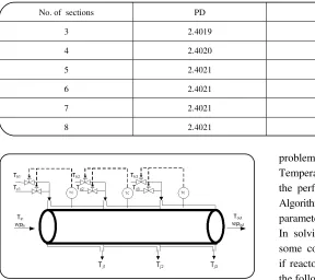
Table 2: Results of reactor temperature optimization for PDref = 2.4 and w = 0.5.

No. of sections PD ωmf PI

3 2.4019 0.0717 0.0026

4 2.4020 0.0696 0.0024

5 2.4021 0.0685 0.0023

6 2.4021 0.0677 0.0023

7 2.4021 0.0672 0.0023

8 2.4021 0.0669 0.0022

Fig.1: Schematic diagram of the reactor.

this index the optimum reactor temperature profile will be obtained.

In [8], reactor wall temperature is chosen as the manipulated variable for temperature control. In [10], for achieving maximum monomer conversion and minimum polydispersity a performance index is defined and using a two-dimensional model, reactor wall temperature has been optimized. In this section, a brief discussion on obtaining the optimal reactor temperature profile is given.

As mentioned above, it is desired to obtain maximum monomer conversion with minimum polydispersity and, therefore the following objective function is considered:

2 2

f ref f ref

PI=w( mω − ωm ) +(1 w)(PD− −PD ) (10)

where ωm is monomer weight fraction, PD is polymer polydispersity and w is a weight factor. Subscripts f and ref stands for final and reference, respectively. For minimizing the above performance index (eq.10), the following three decision variables can be selected.

a) reactor temperature b) reactor wall temperature c) reactor jacket temperature

Therefore, three optimization problems are formulated and discussed below. To solve the first optimization

problem, reactor length has been divided into m sections. Temperatures of these sections are determined such that the performance index (10) is minimized. The Genetic Algorithm Toolbox of MATLAB software with its default parameters are used for performing the optimization task. In solving the above optimization problems, there are some constraints that should be satisfied. For example if reactor temperature is considered as decision variable the following constraints should be taken into account.

100°C <T< 220°C

For other cases, the following constraints on reactor wall and jacket temperatures are considered.

100°C <Tw< 220°C

100°C <Tj< 200°C

It should be noted that in performing optimization on reactor jacket, number of sections, m, is set to three, because according industrial process proposed by Chen [8] the reactor jacket has three heat transfer zones.

Optimization results

In solving optimization problems, as the number of reactor sections increases, it is expected that the discrete profile estimates the continuous profile more closely at the expense of significant raise of computation time. Table 2 and Fig. 2 show effect of number of sections in optimizing of the reactor temperature. As can be seen from Table 2, as number of sections exceeds five, no considerable changes are observed in polymer final characteristics. Therefore, to avoid increase of computation load, five zones have been chosen for further analysis. Effects of weight factor

w

in Tables 3 and 4 and Figs. 3 and 4.

Table 3: Results of reactor temprature optimization using five sections for PDref = PDfeed = 1.9878.

w PD ωmf PI

0.1 2.0149 0.14257 0.0022

0.5 2.0548 0.11725 0.0083

0.7 2.0834 0.10601 0.0099

0.8 2.1066 0.09908 0.0101

0.9 2.1495 0.089528 0.0094

0.95 2.198 0.082083 0.0083

Table 4: Results of reactor temprature optimization using five sections for PDref = 2.4.

w PD ωmf PI

0.1 2.4004 0.0688 0.0005

0.5 2.4021 0.0685 0.0023

0.7 2.4048 0.0684 0.0033

0.8 2.408 0.0683 0.0037

0.9 2.4169 0.0681 0.0042

0.95 2.432 0.0677 0.0044

Fig. 2: Reactor optimal temperature profile using different number of sections for PDref = 2.4 and w=0.5.

on the optimization result. If PDref is chosen to be the same

as feed polydispersity, different weight factors lead into different results. As the value for PDref is increased, effect

of weight factor on the final conversion decreases considerably (Table 4).

The similar results for optimization wall temperature are given in Tables 5 and 6 and Figs. 5 and 6.

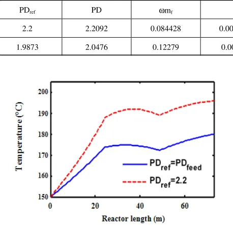
Results of optimization for reactor jacket temperature for w=0.5 and two different polydispersities are shown

in Table and Fig. 7. By comparing results given in Tables 3, 5 and 7, it is concluded that the obtained polydispersity and monomer conversion from the optimal reactor temperature profile are almost the same as those obtained from optimum wall or jacket temperatures Therefore, by applying the optimum jacket temperature, the same results obtained from optimal reactor temperature profile can be achieved.

Dynamic simulation and temperature control

For implementation of the desired optimal temperature profile along the reactor, the following control strategy is applied. The optimum jacket temperature of each section is used as its controller set point of the corresponding zone and the jacket inlet temperatures are considered as manipulated variables. Conventional PID controllers are used for control purposes [16]. For each section of the jacket, hot and cold service fluids are mixed to make the appropriate jacket inlet temperature. In other word, the real manipulated variables are the mass flow rates of hot and cold service streams. Dowtherm A is used as the service fluid inside the jackets.

It is assumed that the inlet feed condition to the reactor is known. This information is sent to a

200

190

180

170

160

150

T

em

p

er

at

u

re

(

°C

)

0 10 20 30 40 50 60 70

Table 5: Results of reactor wall temprature optimization for PDref = PDfeed = 1.9878.

w PD ωmf PI Tω1 Tω2 Tω3

0.1 2.0063 0.15233 0.002646 149.43 125.82 149.11

0.5 2.0476 0.12265 0.009341 164.1 127.36 162.78

0.7 2.0767 0.11064 0.01097 170 128.73 168.7

0.8 2.1003 0.1034 0.011106 173.69 129.87 172.21

0.9 2.1436 0.093624 0.010332 178.99 131.93 176.59

0.95 2.1919 0.086233 0.009158 183.42 133.96 179.33

Table 6: Results of reactor wall temprature optimization problem for PDfeed = 2.4.

w PD ωmf PI Tω1 Tω2 Tω3

0.1 2.4003 0.07356 0.000541 192.14 139.07 182.23

0.5 2.4017 0.07353 0.000541 192.16 139.09 182.23

0.7 2.4037 0.07348 0.003784 192.18 139.13 182.24

0.8 2.4058 0.07344 0.004321 192.21 139.16 182.24

0.9 2.4127 0.0733 0.004852 192.29 139.27 182.25

0.95 2.4235 0.0731 0.005105 192.4 139.44 182.26

Fig. 3: Reactor optimal temperature profile for different values of w and PDref = PDfeed = 1.9878.

Fig. 4: Reactor optimal temperature profile for different values of w and PDref = 2.4.

Fig. 5: Reactor temperature profile using optimum wall temperatures for PDref = PDfeed = 1.9878.

Table 7: Results of reactor jacket temprature optimization for w=0.5.

PDref PD ωmf PI Tj1 Tj2 Tj3

2.2 2.2092 0.084428 0.0036063 191 113.27 174.12

1.9873 2.0476 0.12279 0.009357 165.2 110.07 157.45

Fig. 7: Reactor temperature profile using optimum reactor jacket temprature for w=0.5.

computational unit that calculates set points for the different jacket zones by the a forementioned optimization method. In case of a change in the feed condition or product properties, the optimizer calculates the new optimal jacket temperatures for different jacket zones which are used as set points for the jacket controllers. To simulate the reactor dynamic behavior under control mode, Eqs. 1, 2, 4 and controller equations should be solved simultaneously.

Since the dynamic model is described by partial differential equations, using the orthogonal collocation method [16], the normalized version of equations 1, 2 are descretized in the axial direction as described below. The dimensionless variable x is defined as:

z x

L

= (11)

The normalized version of Eqs. (1) , (2) are given below:

p

m Vz m R

t L x

∂ω ∂ω

= − −

∂ ∂ ρ (12)

p 0 0 j,k

z

2

p i p

R H U (2R )(T T) V

T T

t L x c R c

∆ −

∂ ∂

= − − +

∂ ∂ ρ ρ (13)

k=1,2,...,n

The discritized version of Eqs. (12), (13) are as follows: N 1 p m z m j 1 R (i) d (i) V (i)

A(i, j) ( j)

dt L (i)

+

= ω

= − ω −

ρ (14)

i=2,3,...,N+1 N 1 p z p j 1

R (i) H V (i)

dT(i)

A(i, j)T( j)

dt L c (i)

+

=

∆

= − − +

ρ (15)

0 0 j,k

2

i p

U (2R )(T T(i))

k 1, 2,..., n i=2,3,...,N+1 R (i)c

−

= ρ

The corresponding boundary conditions for different zone are:

1 1 2 2 1 2

2 3

2 2 3 3

m x 1 m x 0 _{m m}

m m

m x 1 m x 0

(N 1) (1)

(N 1) (1)

= = = = ω = ω ω + = ω ω + = ω ω = ω (16) 1 2 2 3

1 x 1 2 x 0 _{1 2}

2 3

2 x 1 3 x 0

T T _{T (N 1) T (1)}

T (N 1) T (1)

T T = = = = = _{+ =} + = = (17)

The resulting ordinary differential Eqs. (4), (14), (15) and controller equation are solved simultaneously.

Model mismatch

In presence of model mismatch, the desired temperature profile can not be established in the reactor because the calculated profile has been obtained from the reactor wrong model. Error in calculating the heat transfer coefficient is a common type of modeling error. To reduce effect of this error, the following correction technique is proposed [16].

1- The temperature at the outlet of reactor is measured. The difference between desired and actual temperatures at the end of reactor is calculated (e_L =T_d,out−T_out).

Errors at the end of each section are estimated using the following equation.

L

i i

e

e z i 1, 2,..., m 1 L

= = − (18)

3- If it is the first trial, by adding the calculated errors to the desired temperatures at the end of each section, the estimated desired temperatures at each section are obtained. A proper curve-fitting method will provide the estimated temperature profile. The mirror image of this estimated profile is the virtual desired temperature profile. In trials other than the first one, the virtual profile is obtained by the same procedure and using the previous virtual profile.

4- Using the virtual optimal temperature trajectory and the reactor model, the corresponding virtual jacket optimal temperature profile is obtained. By discredization this profile into three zones, the new set points for different jacket zones are obtained. After applying these set points by controllers and reaching steady state, the reactor outlet temperature is measured.

5- Steps 1 through 4 are repeated until eL becomes

less than a predetermined value.

Dynamic simulation results

To evaluate the control system performance, feed temperature is decreased to 140°C at t=4500 seconds, and returned to its initial value (150°C) at t=14500 seconds. The results are shown in Fig. 8. As can be seen, after each feed temperature change, the steady reactor temperature profiles are very close to the optimal profile, which demonstrates the effectiveness of the applied control scheme.

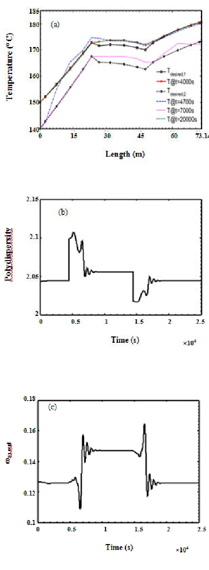
For checking the performance of the proposed control scheme for set point tracking, polydispersity is changed from 2.05 to 2.2 at t=5000 seconds. The results are shown in Fig. 9. As can be seen, the final temperature profile is very close to the optimal profile and the desired polydispersity is almost achieved.

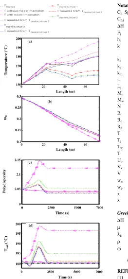
To show the effectiveness of the proposed scheme in case of model mismatch, the simulation results for decreasing the overall heat transfer coefficient by 40%, are shown in Fig. 10. As can be seen the reactor outlet temperature has approached to the optimal outlet temperature and final monomer weight fraction and polydispersity are almost the same as desired ones.

Fig. 9: Closed-loop responses for a change in product polydispersity, Desired profiles and transient reactor temperature b) Polydispersity versus time c) Outlet monomer fraction versus time.

Note: If in addition to monomer conversion and polydispersity ,polymer molecular weight is also to be fixed, one can modify the objective function(5) into the following form:

2 2

1 f ref 2 f ref

PI=w ( mω − ωm ) +w (PD −PD ) + (19)

f 2

3

ref

Mn

w (1 )

Mn

−

As can be seen, the desired number average molecular weight, Mnf, is included in objective function. wis are

weights that can be fixed according to the importance of polymer properties(monomer conversion , polydispersity and molecular weight). For example if one select

1 2 3

1

w w w

3

= = = , and set Mn_ref =92000, ωm_ref =0,

ref

PD =2.45, the optimal wall temperatures will be

Tw1 =172.6, Tw2=155.9, Tw3=181.5. The above

temperatures are used as controller set points.

CONCLUSIONS

Fig. 10: Closed-loop responses for -40% error in heat transfer coefficient; a) Reactor temperature profile variations, b) monomer fraction profiles corresponding to each temperature profile in plot a, c) Polydispersity variations, d) Reactor outlet temperature versus time.

Notations

Cp Specific heat of monomer, polymer or mixture, J/kgK

Cp,j Specific heat of the service fluid

∆H Heat of reaction, J/kg Fj Mass flow rate to the jacket, kg/s

hi Heat coefficient inside the reactor, W/m2K

k Thermal conductivity of polystyrene, styrene or mixture, W/mK ki Initiation rate constant, m6/kg2s

kp Propagation rate constant, m3/s.kg

ktc Termination rate constant, m3/s.kg

L Reactor length, m Lj Jacket length, m

Mn Number average molecular weight, kg/kgmol

Mw Weight average molecular weight, kg/kgmol

N Number of Collocation Points Ri Reactor radius, m

Ro Jacket radius, m

Rp Rate of polymerization

T Reactor's temperature, K Tj Jacket temperature, K

Tw Reactor wall temperature, K

T Time, s Uo External overall heat transfer coefficient, W/m2K

Vz Axial velocity, m/s

V Reactor Volume, m3 wm Styrene weight fraction

wp Polystyrene weight fraction

x Normalized axial position z Axial position, m

Greek Symbols

∆H Heat of reaction, J/kg

µ Viscosity, Pas

λk Rate of k_th moment of polymer distribution

ρ Density of styrene_polystyrene mixture, kg/m3

ω Weighting factor in the objective function

Received : Jun. 14, 2012 ; Accepted : Aug. 26, 2013 REFERENCES

[1] Chen C.C., Continuous Production of Solid Polystyrene in Back-Mixed and Linear-Flow Reactors, Polym. Eng. And Sci., 40, p. 441 (2000). [2] Makwana Y., Moudgalyk K. M., and Khakhar D.V.,

Modeling of Industrial Styrene Polymerization Reactors, Polym. Eng. And Sci., 37, p. 1073 (1997).

200

190

180

170

160

150

T

em

p

er

a

tu

re

(

°C

)

0 20 40 60

Length (m)

0 20 40 60

Length (m)

0 2500 5000 7000

Time (s)

0 2500 5000 7000

Time (s)

0.3

0.25

0.2

0.15

0.1 ωωωωm

2.15

2.1

2.05

0

P

o

ly

d

is

p

er

si

ty

200

195

190

185

180 Tou

t

(°C

)

(a)

(b)

(c)

[3] Bhat S.A., Sharma R., Santosh K., Gupta S.K., Simulation and Optimization of the Continuous Tower Process for Styrene Polymerization, Journal of Applied Polymer Science, 94, p. 775 (2004). [4] Nauman E.B., “Chemical Reactor Design,

Optimization and Scale Up”, McGraw-Hill, (2001). [5] Zhang M., Ray W.H., “Odeling of Living Free-Radical

Polymerization Processes. II. Tubular Reactors, Journal of Applied Polymer Science, 86, p. 1047 (2002).

[6] Beuermann S., Buback M., Gadermann M., Jurgens M., Saggu D.P., Tubular Reactor Synthesis of Styrene-Methacrylate Copolymers in Solution with Supercritical Carbon Dioxide, J. of Supercritical Fluids, 39 , p. 246 (2006).

[7] Agarwal S.S., Kleinstreuer C., Analysis of Styrene Polymerization in a Continuous Flow Tubular Reactor, Chemical Engineering Science, 41, p. 3101 (1986).

[8] Chen C.C., A Continuous Bulk Polymerization Process for Crystal Polystyrene, Polymer-Plastic Technology of Engineering, 33, p. 55 (1994). [9] Chen C.C., Nauman E.B., Verification of a Complex,

Variable Viscosity Model for a Tubular Polymerization Reactor, Chemical Engineering Science, 44, p. 179 (1989).

[10] Costa E.F., Lage P.L.C., Biscaia E.C., On the Numerical Solution and Optimization of Styrene Polymerization in Tubular Reactors, Computers & Chemical Engineering, 27, p. 1591 (2003).

[11] Vega M.P., Lima E.L., Pinto J.C., Use of Bifurcation Analysis for Development of Nonlinear Models for Control Applications, Chemical Engineering Science, 63, p. 5129 (2008).

[12] Wallis J.P., Ritter R.A., Andre H., Continuous Production of Polystyrene in a Tubular Reactor: Part II, AIChE Journal, 21, p. 691 (1975).

[13] Process Economic Program, SRI International, 39D, "Polystyrene", (2001).

[14] Gharaghani M., Abedini H., Parvazinia M., Dynamic Simulation and Control of Auto-Refrigerated CSTR and Tubular Reactor for Bulk Styrene Polymerization, Chem. Eng. Res. Des., doi:10.1016/j.cherd.2012.01.019 (2012).

[15] Hui A.W., Hamielec A.E., Thermal Polymerization of Styrene at High Conversions and Temperatures-An Experimental Study, J. Appl. Polym. Sci., 16, p. 749 (1972).

[16] Shahrokhi M., Nejati A., Optimal Temperature Control of Thermal Cracking Reactor, Ind. Eng. Chem. Res., 41, p. 6572 (2002).