Published online August 10, 2014 (http://www.sciencepublishinggroup.com/j/ajma) doi: 10.11648/j.ajma.20140203.11
Evaluation of kinetic and viscosity based parameters for
fiber reinforced composite rebars at elevated
temperatures: A parametric study
Mohammed Faruqi, Sumon Roy, Francisco Aguiniga, Joseph Sai
Department of Civil and Architectural Engineering, MSC 194, Texas A&M University-Kingsville, Kingsville, TX 78363, USA
Email address:
[email protected] (M. Faruqi)
To cite this article:
Mohammed Faruqi, Sumon Roy, Francisco Aguiniga, Joseph Sai. Evaluation of Kinetic and Viscosity Based Parameters for Fiber Reinforced Composite Rebars at Elevated Temperatures: A Parametric Study. American Journal of Mechanics and Applications.
Vol. 2, No. 3, 2014, pp. 14-20. doi: 10.11648/j.ajma.20140203.11
Abstract:
Fiber reinforced polymer (FRP) composites are high performing materials and offer a wide range of applications. This has led to an increased use of FRP rebars in new construction with concrete as an alternative to steel in buildings. In building applications, FRP rebars need to conform to fire endurance ratings. Unfortunately, there has been very limited effort for understanding the fire endurance of FRP rebars in concrete structures. This limited effort is only available for glass conversion (kinetic parameter) in the glassy state. There is none available for decomposed state (kinetic parameter) and viscosity based parameters influencing the fire endurance of FRP rebars. Moreover, understanding the fire endurance of FRP composite rebars through the standard fire tests is expensive and time consuming. Therefore, this research makes an attempt to develop models that incorporate various transition states of FRP rebars at elevated temperatures to study kinetic and viscosity based parameters. The kinetic parameter in the glassy state is compared with a limitedly available approach in literature. In addition, a parametric study involving decomposed state, and viscosity based parameters in rubbery and leathery states is also carried out to provide some understanding of rebars endurance in fire. A basic understanding is obtained. In order to highlight basic implications on design approaches, a design model is also developed that incorporates the useful transition states in predicting the creep behavior of FRP reinforced concrete structures. This model can serve as a first step in the future design approaches for the construction industry in an economical way.Keywords:
FRP, Elevated Temperatures, Kinetic, Viscosity, Transition States1. Introduction
The use of FRP rebars with concrete in new construction as an alternative to steel has been on rise.High strength to weight ratio and its corrosion resisting properties are superior advantage over steel. FRP reinforcement is used in bridges, multi-storied buildings, parking garages, commercial structures, industrial structures and different types of foundations. Evaluation of kinetic and viscosity based parameters is important at elevated temperatures. This may provide some insight into the stability of rebars to withstand tensile stresses at elevated temperature [1,2]. The behavior of FRP is quite satisfactory and well known at ambient temperatures. At ambient temperatures, when concrete is loaded, an immediate elastic strain develops. However, if this load remains on the structure, creep strains
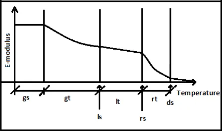
temperature increase. This leads to increased crack-width and deflections at higher temperatures [4,5]. This study is about the elevated temperatures only. Therefore, for the specific examined composite, the viscous flow at ambient temperature is not relevant. However, it may be of interest at elevated temperatures. Unfortunately, these topics have received little attention from research community and therefore lacks insight. This research makes an attempt to develop models that incorporate various transition states of FRP composite rebars in fire to study this. An analytical creep based design approach that incorporates practical transition states is also developed. Figure 1 shows approximate states and polymer transitions at elevated temperatures [6]
Figure 1. Approximate states and transitions of a polymer at elevated temperatures.
gs: glassy state ≤ 100 °C; gt: glass transition zone (approximate); 100 °C ≤ gt ≤ 117 °C; ls: leathery state and glass transition temperature (≈ 117 °C); lt: leathery zone; rs: rubbery state; rt: rubbery zone; 250 °C ≤ rt ≤ 300 °C; ds: decomposed state>300°C.
2. Material and Experimental Setup for
Glass Conversion Parameter
The test setup was reported by Bai et al. [6]. A brief description is provided here for the convenience of the readers. Dynamic mechanical analysis experiments on a pultruded glass fiber-reinforced polyester laminate were performed. The glass transition temperature was reported to be 117 °C. The void content was less than 2%. A 54x12x3 mm3 specimen was subjected to cyclic dynamic loading in a three point bending test using a Rheometrics Solid Analyzer. The specimen was scanned using a dynamic oscillation frequency of 1 Hz. The heating rate was 5 °C/min. The oven was purged with nitrogen during scans. Further details of the experimental setup and testing can be found in [6].
3. Temperature Dependent Kinetic
Conversion Factors
In this analysis, a constant heating rate is assumed. Using Arrhenius equation [7], glassy and decomposed states can
be expressed as: a. Glassy state:
dαg/dT = (Ag/β) exp (-EA.g/RT)(1-αg)n (1) b. Decomposed state:
dαd/dT = (Ad/β) exp (-EA,d/RT)(1-αd)n (2)
3.1. Kinetic Parameters at the Glassy State
The kinetic parameters in the glassy state can be estimated using an extension of Arrhenius equation. A constant heating rate is assumed. This yields:
dα /(1-αg) = (Ag/β) , / dT (3) To simplify the prediction of αg, we linearize equation (3) using Taylor series, and for n= 1 andαg < 1 the equation becomes:
-ln(1-αg)/T2
=
(AgR/βEA,g)*(1-2RT/EA,g)*exp(-EA,g/RT) (4) Considering ‘ln’ of both sides of equation (4) provides:ln(-ln(1-αg)/T2) = ln[(AgR/βEA,g)*
(1-2RT/EA,g)*exp (-EA,g/RT)] (5) Various constants for use in later calculations can be obtained from [6,7].
They are: EA,g = 74.30 kJ/ mol;
Ag = (141± 1.52)*107; R = 8.314 J/mol K and β ≈ 3.65*105 J/min
Taylor’s series expression can be used to expand ln(1-αg). This yields:
ln(1-αg) = - αg - αg2/ 2 - αg3/3 + --- (6) if -1< αg < 1
Multiplying both sides of equation (6) by –1, provides: -ln(1-αg) = αg + αg2/ 2 + αg3/3 + --- (7) Ignoring higher order of αg provides:
-ln(1-αg) = αg (8) Again considering ‘ln’ of both sides of equation (8) yields:
ln(-ln(1-αg)) = ln(αg) (9) The right-hand side of equation(9) after expansion by Taylor series provides:
ln(αg) = 2[(αg-1)/(αg+1) + 1/3{(αg-1)/(αg+1)}3 + 1/5{(αg-1)/(αg+1)}5 + ---] for αg >0 (10) Neglecting higher order of the expansion in equation (10) and simplifying yields:
- 2[(1- αg)/(1+ αg)] = - 2[(1- αg)(1+ αg)-1] (11)
Expansion of (1+ αg)-1 into equation (11) yields: (1+ αg)-1 = 1 – αg – αg2 – αg3 – --- (12)
Neglecting the higher orders of αg in equation (12) provides: (1+ αg)-1 = (1 – αg) (13)
Substituting equation (13) into equation (11) provides the following: ln(αg) = –2(1– αg)2 (14)
Equating equation (5) and (9) provides: ln(αg ) = ln[(AgRT2/βEA,g)*(1-2RT/EA,g)*exp(-EA,g/RT)] (15) Equating equations (14) and (15) yields: –2(1–αg)2=ln[(AgRT2/βEA,g)* (1-2RT/EA,g)]-(EA,g/RT) (16) The values of αg are computed and a comparison is shown in Figure 2. Figure 2. Glass conversion degree ratios vs.temperature. 3.2. Kinetic Parameters at the Decomposed State The kinetic parameters in the decomposition state are estimated using: dαd/dt = (Ad / β) exp (-EA,d / RT) (1-αd)n (17)
To predict conversion degree (αd) at decomposed state, we apply Taylor’s series to equation (17). Considering n = 1.0 for a single order equation yields: dαd / (1-αd) = (Ad/β) , / dT (18)
Integrating left-hand side from rubbery to decomposed state and right-hand side from the actual time to the decomposition at infinity provides: dα /(1-αd)=(Ad/β) , / dT (19)
Equation (19) after simplification yields: ln [(1-αd) / (1-αr)] = (AdRT2/βEA,d)* (1-2RT/EA,d)*exp(-EA,d/RT) (20)
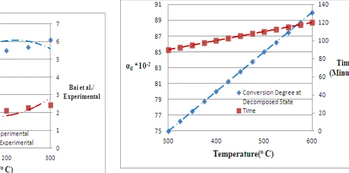
At the decomposed state, rubbery conversion degree does no longer exists. Therefore, it can be assumed that αr = 0 and EA,d = 80.1 kJ/mol K and β = 4.265*108 J/min [7]. Multiplying both sides of equation (20) by -1 yields: -ln (1-αd) = - (AdRT 2 /βEA,d)*(1-2RT/EA,d)*exp(-EA,d/RT) (21) Linearizing left side of equation (21), ignoring high order of αd, and equating with equation (20), provides: αd = -(AdRT2/βEA,d)*(1-2RT/EA,d)*exp(-EA,d/RT) (22) Considering ‘ln’ of both sides of equation (22) and simplifying yields: Ln(αd) = ln[-{(AdRT2/βEA,d) *(1-2RT/EA,d)*{exp(-EA,d/RT)}] (23) Depending on the nature of fire, the decomposed state of FRP material usually occurs between 90-120 minutes of fire [8-10]. A parametric plot is shown in Figure 3. Figure 3. Temperature, time, and decomposed state conversion degree.
4. Viscosity
Viscosity is an indicator of the resistance to flow. All plastics are non-Newtonian. This means that their viscosity does not remain constant over a given range of shear. 4.1. Estimation of Volume Changes with the Rise in Temperature Assuming a unit volume of initial material at a specified temperature, the volume of the material at the different states can be expressed as follows [6,7,8]: Λg = (1-αg) (24)Λl = αg (1- αr ) (25)
Λr = αg αr (1- αd) (26)
4.2. Modeling of Temperature-Time Dependent Viscosity
As the temperature rises, four different material states may be found at different temperature regimes. The material viscosity is a function of temperature and time and as a result viscosity in the four states is different. In other words, µm = f(T, t)
These states are characterized as follows:
µm = µg + (µl - µg)αg +(µr -µl) αg αr + (µd - µr) αg αrαd (28) The maximum value of viscosity can be obtained by partial differentiation of the material viscosity with respect to temperature and time. Partially differentiating equation (28) with respect to temperature and time, and considering µl > µg ; µl > µr and µr > µd yields:
∂2µm/(∂T∂t) = µl ∂2αg/(∂T,∂t) –
µl∂2(αgαr)/(∂T∂t)–µr∂2(αgαrαd)/(∂T∂t) (29) Maximum viscosityat a specific temperature and time domain is provided by:
∂2µ
m/(∂T∂t) = 0 (30) Therefore, equation 29 yields the following:
µl ∂αg/(∂T∂t) - µl ∂(αgαr)/(∂T∂t) – µr∂(αgαrαd)/(∂T∂t) = 0; This simplifies to:
µl∂2 {αg(1-αr)}/(∂T∂t) – µr∂2(αgαrαd)/(∂T∂t) = 0 (31) Substitution from equations (24) and (26) into (31) and dividing by µlµr yields:
(1/ µr) ∂2Λl/(∂T∂t) –(1/ µl)∂2Λd/(∂T∂t) = 0 (32) Integrating equation (32) with respect to time and temperature provides:
(1/µr) { l/∂T∂t}dTdt
– (1/µl) { d/∂T∂t}dTdt = 0 (33)
From a practical design scenario, the glass to leathery state occurs between 30 to 60 minutes of heating and rubbery to decomposed state in the range of 90 to 120 minutes. The heating rate ranges from 2.5oC/minute to 5 o
C/minute [9, 10-11]. Therefore,
(1/µr) { l/∂T∂t}dTdt
– (1/µl) { d/∂T∂t}dTdt = 0 (34)
Integration, simplification, and re-arranging of equation (34) yields:
µl/ µr = (Λd – Λr)/ (Λl – Λg) (35) Volume fractions at glassy state is about 30%. For
leathery, rubbery, and decomposed states, it respectively varies from 60% to 75%, 75% to 90%, and 100% [9,12-13]. The viscosity at leathery state is approximately around1.6*108 Poise [6, 8]. Basic parametric comparisons are shown in Figures 4, 5, and 6.
Figure 4. Rubbery viscosity and the ratio of rubbery viscosity to leathery vs. temperature.
Figure 5. Rate of change of material viscosity with respect to time and temperature.
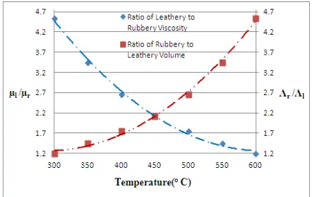
Figure 6. Ratios of leathery to rubbery viscosity and rubbery to leathery volume vs. temperature.
5. Creep Based Design
design approaches. Temperature is a factor as the FRP rebars must stay below the glass transition temperature to hold its properties.
5.1. Formulation of E-Modulus
The E-modulus of FRP can be calculated as follows: A unidirectional composite can be modeled by assuming fibers to be continuous and parallel throughout the composite. This model is shown in Figure 7.
Figure 7. Model of unidirectional composite.
σfrp= σf(Af/Afrp) + σm (Am/Afrp) (36) Equating area fractions to volume fractions, differentiating with respect to strain, substituting E-moduli, and substituting Elt Vlt for Εm Vm due to temperature effects into equation (36).
Efrp = EfVf + Elt Vlt (37)
5.2. Development of Creep Model at Elevated Temperatures
At higher temperatures and sustained loads, the concrete shrinks, and produces cracks. This causes the FRP rebars in the beam to be compromised. This creep deflection depends
on creep curvature and the
support conditions of FRPreinforced concrete system. This can be expressed as:
∆cr = Ss λcr L (38) λcr = 3.5 The/( Econc Ieff ) (39) Th = Afrp εh EFRP (40) Substitution of Th and λcr into equation (40)
∆cr ={ 3.5SseL/Ieff }[{Afrp εh Efrp}/Econc ] (41) Material volume [6] at a practical state can be obtained as:
Vf = (1- αg) and Vlt = (1- αg) (42) Substituting the volumes provides:
Efrp = Ef (1-αg ) + Elt ( 1- αg ) (43) Placing equation (43) into equation (41) provides:
∆cr = [{3.5SseL Afrp εh }/Ieff]*
[{Ef (1-αg ) + Elt ( 1- αg )}/Econc] (44)
6. Comparison of Results and
Discussion
A parametric study and a design approach is carried out. The results of glass conversion are shown in Figures 2. Decomposed conversion is shown in Figure 3. In Figure 2, the glass conversion degree ratios predicted using the model are closer to experimental values as opposed to the literature model. The model and literature ratios respectively range from 0.52 to 0.90 and 4 to 2.8 for a temperature range of 0 to 300 °C. In Figure 3, as the temperature increases, the conversion degree at decomposed state also increases. At a temperature of about 550 °C and a time of about 118 minutes, the decomposed conversion degree reaches about 88% of de-gradation. This implies that most of the resin is burnt out.
The results of viscosity based analysis are shown in Figures 4, 5, and 6. In Figure 4, as the temperature increases the rubbery viscosity exhibits lower viscosity. Accordingly, the rubbery and leathery viscosity ratio increase. This ratio ranges from 0.22 to 0.82 for a temperature range of 300 to 600 °C. An inflection point (concavity of the curve) is formed at a temperature of approximately 435 oC and µr ≈ 3.67 x 10⁶ Poise. Using basic graph geometry, approximate slopes before and after the inflection points for the rubbery viscosity are found to be respectively 2.2 and 1.1 %. This shows that the conversion rate of rubbery viscosity to being less viscous (more fluidity) is much higher before the inflection point and starts to decrease after an approximate temperature of 435 oC. Figure 5 shows the rate of change of material viscosity with respect to time and temperature. The approximate rate decreases from 3.33 to 0.45 *103 Poise/ o
C/min respectively before and after inflection point. The rate at the inflection point is about 1.58*103 Poise/ oC/min corresponding to an approximate temperature and time of 430 oC and 80 minutes. The rate of change of material viscosity seems to be lower after the inflection point with temperature increase. This can be attributed to the fact that most of the composite material is already in liquid form before the inflection point and as a result the conversion rate slows down. Figure 6 shows the ratios of leathery to rubbery viscosity and rubbery to leathery volume with respect to temperature. Approximate slopes for the ratios of leathery to rubbery viscosities are respectively 1.61 and 0.61% before and after the inflection point of curve. The approximate inflection point for this plot is 450 oC. This again shows the conversion rate seems to slow down within the vicinity of inflection point. The opposite is true for the ratios of rubbery to leathery volume.
7. Conclusions and Future Work
In this research paper models that incorporate different transition states of FRP composite rebars in fire to parametrically provide an insight into temperature dependent kinetic and viscosity based parameters are developed. An analytical creep based design approach is also developed. Based on the information presented in this paper, the following basic conclusions can be drawn:
1. The predicted glass conversion degree ratios are conservative.
2. As the temperature and time increase, the decomposed conversion degree also increases. At approximately 90 and 118 minutes, the decomposed conversion degrees are respectively 85% and 88% of the original.
3. The conversion rate of rubbery viscosity to being less viscous is much higher before the inflection point and starts to decrease after an approximate temperature of 435 oC.
4. The rate of change of material viscosity seems to be lower after the inflection point with temperature increase. The rate at the inflection point is about 1.58*103 Poise/ oC/min.
5. The ratios of leathery to rubbery viscosity and rubbery to leathery volume respectively seem to decrease and increase with temperature increase. The conversion rate of leathery to rubbery viscosity seems to slow down within the vicinity of the inflection point. The approximate inflection point occurs about450 oC. 6. A basic creep based design approach is developed.
This can serve as a first step in the future design approaches for the construction industry in an economical way.
7. A basic understanding of the behavior of kinetic and viscosity based parameters together with a first step creep based design approach can provide some insights into enhancing the fire endurance of FRP composite rebars and may be helpful in the future design approaches for the construction industry in an economical way. However, there is much room for refinement to the initial work performed here. Future work may include to develop 3D nonlinear finite element models (14) that are capable of predicting such parameters and using them in an experimentally verified creep based design approach.
Notations
Af Area of fibers
Afrp Tension reinforcement
A Pre-exponential factor of glass state Am Area of matrix
A! Pre-exponential factor of rubbery state
A Pre-exponential factor of decomposed state
E#, The activation energy at glass-transition
E#,! The activation energy at leather to rubbery transition
E#, The activation energy at rubbery to decomposed transition
Econc Young’s modulus of concrete Ef Young’s modulus of fibers Efr Young’s modulus of FRP rebar
E$ Young’s Modulus of the material
E Young’s Modulus of glassy state Elt Young’s modulus in the leathery zone
E! Young’s Modulus of rubbery state
E Tension reinforcement to neutral axis distance Ieff Effective moment of inertia
L Beam span
Ss Support conditions of the FRP system exposed to elevated temperatures
N The reaction order
R Universal gas constant (8.314 J/mol K)
T Temperature
Tm Temperature of the material Th Tension force due to creep
T Time
tg Time at glassy state tl Time at leathery state Vf Volume of fibers
Vlt Volume in the leathery zone
αg Conversion degree of glass-transition (kinetic parameter at glassy state)
α Conversion degree of rubbery to decomposed state (kinetic parameter at decomposed state)
α! The conversion degree of leathery to rubbery state of polymer
β Constant heating rate
∆cr Creep deflection at elevated temperature Λ The content of the material by volume Λg The content of the materials at glassy state Λl The content of the materials at leathery state Λr The content of the materials at rubbery state Λd The content of the materials at decomposed state εh Concrete strain due to elevated temperature λcr Creep curvature
µm Material viscosity µg Viscosity at glassy state µr Viscosity at rubbery state µl Viscosity at leathery state
µd Theoretical viscosity at decomposed state σf Stress in fibers
σfrp Stress in FRP rebar σm Stress in matrix
References
[1] Keller, T.; Tray, C.; Zhou, A. Structural Response of liquid-cooled GFRP slabs subjected to fire. Part I: Material and post-fire modeling, Composites Part A. 2006, 37(9), 1286-95.
[3] Dao, M.; Asaro, R. A study on the failure prediction and the design criteria for fiber composites under fire degradation,
Composites Part A. 1999, 30(2), 123-31.
[4] Bausamo, J.; Boyd, J.; Lesko, J.; Case, S.W.Composite life under sustained compression and one-sided simulated fire exposure: Characterization and prediction, Proceedings of the International SAMPE Symposium, Long Beach, USA, 2004.
[5] Halverson, H.; Bausano, J.; Case, S.W.; Lesko, J. Simulation of response of composite structures under fire exposure,
Proceedings of the International SAMPE Symposium, Long Beach, USA, 2004.
[6] Bai, Y.; Keller, T,; Valle, T. Modeling of stiffness of FRP composites under and high Temperatures, Composites Science and Technology, 2008, 68, 3099-3106.
[7] Davis, R.E. Modern Chemistry, Harcourt Brace & Company, Boston, MA, 1999.
[8] Bai, Y.; Valle, T.; Keller, T. Modeling of thermo-physical properties for FRP composites under elevated and high temperatures, Composites Science and Technology, 2007,
67(15-16), 3098-109.
[9] Mahieux, C. A.; Reifsnider, K.L. Property modeling across transition temperatures in polymers: a robust stiffness--temperature model, Polymer, 2001, 42, 3281-91.
[10] Schapery, R. Thermal expansion co-efficients of composite materials based on energy principles, Journal of Composites Material, 1968, 2(3), 380-404.
[11] Katz, N.; Berman, N.; Blank, L. Effect of high temperature on bond strength of FRP rebars, Journal of Composites for Construction, 1999, 3(2), 73-81.
[12] Mahieux, C. A. A systematic stiffness-temperature model for polymers and applications to the prediction of composite behavior, Ph.D., dissertation, Virginia Polytechnic Institute and State University; 1999.
[13] Mahieux, C.A.; Reifsnider. K.L. Property modeling across transition temperatures in polymers: application to thermoplastic systems, Journal of Material Science, 2002,
37, 911-20.