Douglass et al.EPJ Data Science (2015) 4:4 DOI 10.1140/epjds/s13688-015-0040-6
R E G U L A R A R T I C L E
Open Access
High resolution population estimates
from telecommunications data
Rex W Douglass
1,2*, David A Meyer
1,2, Megha Ram
2, David Rideout
1and Dongjin Song
1,2,3*Correspondence:
1Department of Mathematics,
University of California/San Diego, La Jolla, CA 92093, USA
2UC Institute on Global Conflict and
Cooperation, La Jolla, CA 92093, USA
Full list of author information is available at the end of the article
Abstract
Spatial variations in the distribution and composition of populations inform urban development, health-risk analyses, disaster relief, and more. Despite the broad relevance and importance of such data, acquiring local census estimates in a timely and accurate manner is challenging because population counts can change rapidly, are often politically charged, and suffer from logistical and administrative challenges. These limitations necessitate the development of alternative or complementary approaches to population mapping. In this paper we develop an explicit connection between telecommunications data and the underlying population distribution of Milan, Italy. We go on to test the scale invariance of this connection and use telecommunications data in conjunction with high-resolution census data to create easily updated and potentially real time population estimates in time and space.
Keywords: cell phone network; gravity model; scale invariance
1 Introduction
Census data help us understand patterns of human development and movement. Spatial variations in the distribution and composition of populations inform urban development, health-risk analyses, disaster relief, and more. Despite the broad relevance and importance of such data, acquiring local census estimates in a timely and accurate manner is chal-lenging because population counts can change rapidly [, ] and are contingent on public participation [, ]. Moreover, censuses are expensive [, ], can be politically charged [, ], and suffer from logistical and administrative challenges [, ]. These limitations necessitate the development of alternative or complementary approaches to population mapping.
Telecommunications data like cell phone calls, text messaging, and internet use are a promising new source of real-time measure of population. In Figure , data on aggregate call volume and internet use in Milan, Italy can distinguish days of the week, holidays, and important events. The data clearly display daily and weekly rhythms with most telecom-munication during daytime, high levels on weekdays, less on Saturdays, and even less on Sundays. They also identify significant holidays, in this case with an unusual calling pattern during the week of Christmas and New Year’s Eve. The data even attest to the importance of soccer in Milan, as a spike in internet usage on December , coincides with the World Cup Draw. Telecommunications data clearly encapsulate important information
Figure 1 Hourly telecommunications activity for Milan, Italy.
about behavioral patterns and social phenomena, so it is reasonable to use these data to map selected aspects of Milan’s social geography.
In this paper we use telecommunications data in conjunction with census data and satel-lite images to create high-resolution population estimates in time and space. The next section details existing approaches. We then describe new data on telecommunications activity from Milan, Italy, a unique land cover measure developed using recent satellite images of the region, and a recent national census. The first empirical section investigates the proportionality of calling activity to population and how it varies over different geo-graphic scales. We then propose and evaluate several models for predicting the population of a given area and the percent of that population which is of foreign nationality. We con-clude with a discussion of the benefits and limitations of our approach and propose ways it could be used in real inter-census population estimation.
2 Related work
Other sets of telecommunications data have been used to study population density and distribution [–], detect community networks [–], and map mobility patterns [–]. Some studies have assumed a connection between telecommunications data and population—two examples include Girardinet al., who use phone data as a proxy for pop-ulation [], and Readeset al., who take the spatial and temporal distribution of telecom-munications activity to indicate urban activity []. In this paper, however, we develop an explicit connection between call data and the underlying population distribution.
Kringset al. analyze this connection and show that call volume scales linearly with popu-lation [], a result we reproduce at certain geographic scales with the data for Milan. Kang et al. explored this connection further: they compute a correlation coefficient of . be-tween call volume and the underlying population distribution by comparing LandScanTM’s
in-Douglass et al.EPJ Data Science (2015) 4:4 Page 3 of 13
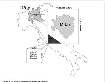
Figure 2 Region of interest and unit of analysis.
variance above certain levels of aggregation. We are thus able to predict population distri-bution at a resolution of m× m for much of Milan which is a finer resolution than the popular LandScanTMwhich provides population estimates at a resolution of km.
The work most similar to our analysis is provided by Devilleet al. who use a combi-nation of telecommunications data and remote sensing to develop m× m pop-ulation estimates for France and Portugal []. Their focus is primarily on downscaling known population from larger census tracts to smaller grid units, and they estimate a fixed proportionality between nighttime call activity and population. Our focus is on predict-ing population with models trained on known census data but applied to an inter-census period. Because this is a more problematic task, we are interested in variation in the pro-portionality of telecommunications activity and population, broken down across multiple types and times of activity, and with potential interactions with remote sensing data like land use.
3 Description of the data
Our region of interest is a . kmsquare area in the Lombardy region in northern Italy,
Figure . It encompasses Milan, the second largest city in Italy, towns with populations greater than ,, and large stretches of rural farmland and commercial areas. Our units of analysis are a regular grid of m by m cells (, in total), dictated by the resolution of the telecommunications data provided by Telecom Italia as part of the Big Data Challenge, described in detail below.
classifica-Figure 3 Land use estimate for region. (a)Landsat 8 pansharpened natural color satellite image of region.
(b)Land use classification: water (blue), agriculture (green), buildings (brown), roads (grey), rail roads (black).
tion is directly available for % of our area from polygon and line layers from the Open-StreetMap database []. To classify the remaining % we employ m resolution pan sharpened natural color Landsat satellite imagery, shown in Figure (a). We train a ran-dom forest classifier using OpenStreetMap data as labeled training examples.bThe final
classifications for each pixel is shown in Figure (b). We estimate that the region is pri-marily covered in vegetation (%), followed by structures (%), road/pavement (%), rail (%), and water (%).
Our main outcome of interest is population, the number of total persons living in a given area, and foreign population, the number of foreign nationals. Our population measures come from the National Institute of Statistics (Istituto Nazionale di Statistica).cThe Cen-sus of Population and Housing provides demographic data forsezioni, or census sec-tions. These population counts are geographically mapped according to ISTAT territorial bases. There are ,sezionithat intersect our region of interest. The census tracts are irregular polygons of varying shapes and sizes. We divide the population in eachsezione uniformly across the area it covers, sum within each grid square, and round to the nearest individual for the final population estimate.
The distribution of population is bimodal, shown in Figure (a). Population is dis-tributed exponentially for small values with % having zero population, % having a pop-ulation of , % with a poppop-ulation of , and so on. Thirty-nine percent of grid-squares have a population over and approximately follow a log normal distribution with a mean of persons. The geographic distribution of population is shown in Figure (b).
Our measures of telecommunications activity are provided by Telecom Italia as part of the Telecom Italia Big Data Challenge.dThe Call Detail Records (CDRs) aggregated in the
Douglass et al.EPJ Data Science (2015) 4:4 Page 5 of 13
Figure 4 Distribution of population. (a)Distribution of 2011 census population interpolated to grid squares.(b)Population density across region.
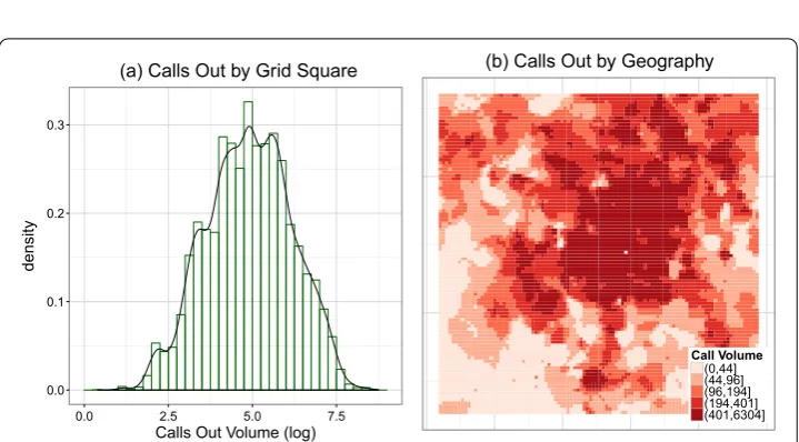
Figure 5 Distribution of calling activity. (a)Distribution of total call volume (CALLOUT) by gridsquare.(b)
Geographic distribution of call volume (CALLOUT).
each of the m× m meter grid cells. The activities are further disaggregated by country codes that indicate the country of origin (in the case of incoming calls and texts) or destination (in the case of outgoing calls and texts).
The original dataset contains ,, entries, each of which includes data for all telecommunication types, for a distinct minute time slot, country code, and grid square. We generate several aggregations for each of the five activities including total over the en-tire period (), total by time of day by hour (), and total by country code ().e
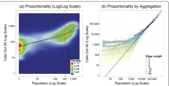
Figure 6 Scale variance of the relationship between population and calling activity. (a)Proportionality of call volume (CALLOUT) to population. Fits shown include linear trend (black), piecewise linear trend with an estimated structural break at 351 persons (red), and LOESS curve with 95% confidence intervals (blue).(b)
Proportionality of call volume and population at larger geographic aggregations of size 1×1 grid squares, 2×2 grid squares, etc. LOESS curve fit to each separately with 95% confidence intervals. A 45 degree line (black) shows linear proportionality for comparison.
4 An elementary model
Previous analyses of telecommunications data have shown that call volumes,wi, associated with a location/regioniscale with the populations,pi:wi∝pα
i [, ]. Equivalently,
logwi=b+αlogpi. ()
We begin by finding the parametersbandαso that () best fits population and total call data. More precisely, since the total SMSIN, SMSOUT, CALLIN, CALLOUT, and INTERNET volumes have correlations of ., ., ., ., ., with popu-lation, we letwibe the total CALLOUT volume for grid squarei. That CALLOUT is best correlated with grids quare population is consistent with analyses of other telecommuni-cations datasets [, ]. The results of a linear regression, a piecewise linear regression, and LOESS curve appear in Figure (a). If call volume and population were proportional, these points would lie on a degree line. The expected linear fit (black) fits the data rather poorly. Instead, a LOESS curve (blue) better captures the changing proportionality, which we can further approximate with a piecewise linear fit with an estimated structural break at persons. That is, in contrast to previous work, we find a linear proportionality only above a certain threshold of population, a slope . (% CI of .-.), but below that threshold the fit and the trend substantially weaken to only . (% CI of .-.).
Douglass et al.EPJ Data Science (2015) 4:4 Page 7 of 13
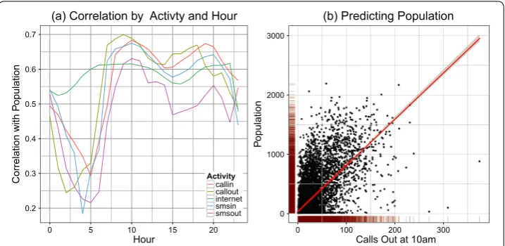
Figure 7 Bivariate relationship between population and telecommunications activity disaggregated by hour. (a)Bivariate correlation between telecommunications activity at a particular hour and population.
(b)Population as a function of call volume (CALLOUT 10 am). Linear fit (red) with 95% confidence intervals.
where there are more towers, the relationship would be easier to observe in dense areas and weaker in less dense areas.
To test for this possibility, we generate synthetic grid squares at larger levels of aggre-gation. The nonoverlapping tiles begin with edge length of which is the original m aggregation, edge length of is twice that at m, and doubling accordingly up to by grid squares. Figure (b) shows the change in log population relative to log call volume with points colored by their level of aggregation and a LOESS curve with % confidence intervals. If the relationship were only scale driven, larger aggregations with population above persons should be distributed around the degree line of proportionality one. Instead, each level of aggregation shows a hook pattern, shifting to a proportionality of above some population size except for very large aggregations which lie almost entirely on the degree line. This relationship supports the view that, regardless of aggregation, there is something different about measurements from sparse areas. It also demonstrates why other studies depending on larger levels of aggregations would show near proportion-ality averaging over the difference between kinds of areas.
That the estimated slope in () is not significantly different from (above a relatively small threshold) justifies the use of a simple model in whichwi∝pi, or equivalently,
pi=mwi, ()
where we have written () with the populations on the right hand side because our goal is to use call volumes,wi, to estimate populations,pi.
call volumes, CALLOUT has the greatest correlation, approximately .. Thus we use CALLOUT from am to am for thewiin ().
Figure (b) shows populations plotted as a function of CALLOUT volume from am to am,i.e., a transposed, unlogged version of Figure (a). The red line is the least squares fit to model (); it has slope .±.; the RMS error is approximately persons; and it has anRof ..
5 Toward real time population estimates
While the next census won’t be available until , telecommunications data combined with readily available mapping and land cover data can potentially provide highly accurate and nearly real-time monitoring of population growth and migration. Such data facilitate standard applications of census data, such as the planning and provision of services, by producing up-to-date population data in between census years. High-resolution popula-tion estimates in real-time are especially useful in scenarios that require a time-sensitive understanding of population distribution and density. For example, emergency planning utilizes data on physical landscapes and hazards as well as on population to create opera-tional evacuation plans. Change in the size or distribution of sub-populations impacts the viability of evacuation plans; up-to-date population data can thus complement traditional census data to make emergency planning more effective [].
Developing such an estimator requires building a model that has both high predictive accuracy and generalizes without overfitting the data. Additionally, the above analysis sug-gests several desirable properties and motivates the need to move away from a simple ordinary least squares framework. First, because proportionality of calls to population is approximately linear only above a certain density of population, our model will need to account for nonlinearities, discontinuities, and nonmonotonic relationships. Second, we speculate that the proportionality should vary with factors such as urbanity which could be captured with measures of land use, so the model needs to be able to test for complex interactions. Third, there is additional information in call activity at other times of day that might help distinguish between commercial and residential areas, so the model will need to able look for those signals among hundreds of correlated features.
One method that meets all of these criteria is a random forest regression, which com-bines the strengths of ensembles, bagging, and nonparametric binary trees []. A random forest is an ensemble of fully grown decision trees, each fit to different random subsets of the data and with a random subset of features. For each tree, the data are randomly par-titioned into a training sample that includes two-thirds of the observations and an out of sample test set that includes the remaining third. Each tree is then constructed iter-atively, selecting cut points that partition the training set into increasingly pure subsets with respect to the outcome variable. Because our data are spatially correlated, we further partition our data with -fold cross validation, each time holding back a spatially con-tiguous section of one-tenth of the region []. For each fold, we fit trees. For variable importance, we report the median and spread across all folds. For predictive accuracy, we report the root mean squared error (RMSE) for predictions made on the spatially con-tiguous hold out test set for each fold.
Douglass et al.EPJ Data Science (2015) 4:4 Page 9 of 13
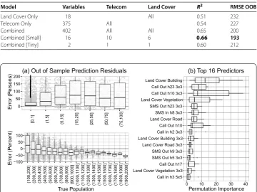
Table 1 Model results: Total population
Model Variables Telecom Land Cover R2 RMSE OOB
Land Cover Only 18 All 0.51 232
Telecom Only 375 All 0.54 227
Combined 402 All All 0.65 200
Combined [Small] 16 10 6 0.66 193
Combined [Tiny] 2 1 1 0.60 212
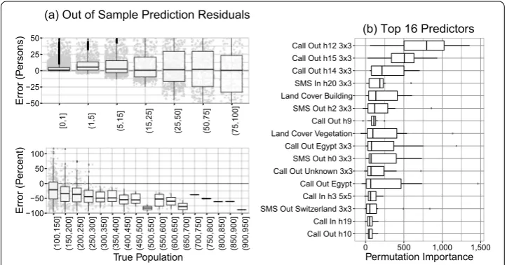
Figure 8 Total population model (random forest, top 16 predictors, Combined [Small] model). (a)Residuals in number of persons for true population under 100 and in percent error by true population over 100.(b)Boxplot of permutation importance for features across each of 10 spatially contiguous holdout test sets during cross-validation.
railroads and measured at three different levels of spatial aggregation, ×, ×, and × grid squares. The telecommunications measures include each of the five activities broken down by hour of day and again measured at three different spatial aggregations. In-dividually, both the land cover measures and telecom measures have comparable accuracy with a RMSE of persons and persons. Combining the two results in a substantial % reduction in RMSE to persons.
A fourth model is a subset of the combined model, keeping only the most important variables identified by a procedure introduced by []. Focusing on only a subset of im-portant variables further improves the out of sample accuracy to a RMSE of persons. This is an improvement on the baseline OLS benchmark by %. Figure (a) shows the prediction accuracy and how it varies by the size of the true population. The model over-estimates small populations and underover-estimates larger populations.fThe variance is also larger for less populated areas.
Figure 9 Predicted population as a function of calls out at 10 am and building land cover from Combined [Tiny] random forest model. (a)Marginal effects, predicted population setting the variable at a fixed level and holding the rest of the dataset at their observed values. Shown are the mean prediction (black) and 95% confidence interval of the mean (red).(b)Joint effects, predicted population varying both calls out and land cover together.
those that contribute unique information not found elsewhere (e.g. calls out made at pm, text messages received at am, and calls in at am).
A fifth model includes only the top two predictors: calls made out at am and building land cover. Just these two variables are sufficient to provide a RMSE of persons. To better understand how they help capture population, Figure (a) shows their marginal effect and Figure (b) shows their joint effect. Greater call volume out at am has a clear positive association with population. In contrast, the percentage of a gridsquare covered by buildings has a non-monotonic and conditional relationship with population. The most populated areas are those with both high levels of buildings and high call volume. Areas with a great deal of buildings (over %) but little calling activity, however, are sparsely populated and likely commercial or industrial areas.
6 Documenting immigrant populations
According to the National Institute of Statistics (Istituto Nazionale di Statistica), the for-eign resident population was nearly .% of the total population of Milan on January , .gSome of these immigrants form geographically concentrated communities while others are distributed more evenly throughout the city []. Moreover, some migrants are irregular (illegal) and thus complicate efforts to compile population data []. The increas-ing number of immigrants to Italy, both regular and irregular, has led Italy to tighten its migration and integration policies as well as to institute a number of amnesty programs in recent decades [].
Douglass et al.EPJ Data Science (2015) 4:4 Page 11 of 13
Figure 10 Foreign population model (random forest, top 16 predictors). (a)Residuals in number of persons for true population under 100 and in percent error by true population over 100.(b)Boxplot of permutation importance for features across each of 10 spatially contiguous holdout test sets during cross-validation.
on Undocumented Migrants,ithe European Programme for Integration and Migration,j and more - that work on behalf of these migrants.
As before, we fit a random forest regression with -fold spatially-contiguous cross-validation. We start with the full set of land use measures, the full set of telecommunica-tions measures, and include additional measures of each communicatelecommunica-tions activity broken down by the target country. Again we cull the model, coincidentally also leaving key variables. The model has an RMSE of foreign born persons, and anR of .. The
model tends to over-predict in areas with few foreigners and greatly under-predict the number of foreigners with populations of or more, Figure (a). Figure (b) shows the permutation importance of each variable and highlights the utility of including mea-sures of international communications. Calls out to other nations, in particular Egypt and Switzerland, are strong indicators of foreign populations in and around Milan. Other countries which were flagged as important for some geographic folds but not the entire region include Peru, Sénégal, and China. Not only do these records indicate where im-migrant populations live in and around Milan, they plausibly could indicate the specific ethnic origin.
7 Discussion
We have also shown, however, that telecommunications activities are most useful in context, in conjunction with other spatial measures of human activity, tuned to local con-ditions. Model parameters developed for one region or country would likely be inappro-priate if applied blindly to another. In each application, a baseline model should be estab-lished with a recent census. Once a baseline model is estabestab-lished, it will need to be recal-ibrated over time. As mobile phone market penetration and usage patterns change, the relationship between telecommunications activity and population will also change. We envision an inter-census calibration using a very small scale stratified population count in key calibration regions. Inter-census calibration could also be supported by direct es-timates of changing market penetration and use patterns as well as additional annually updated population proxies such as tax records. Further, population estimates are typi-cally extrapolated based on long term growth rates. How estimates based on real-time telecomunications measures compare to or improve those estimates is an open question for future research.
Competing interests
The authors declare that they have no competing interests.
Authors’ contributions
The authors worked together to complete the Telecom Italia Big Data Challenge project upon which this paper is based. MR conceived the question of estimating (sub)populations, acquired the population registrar data, and researched practical applications of our method. RWD and DR acquired and processed the telecommunications data. MR acquired the GIS data and RWD processed it. DAM and RWD developed and implemented the baseline and extended high-resolution population estimation procedures, respectively, in consultation with the other authors. RWD developed the land use measures, random forest estimations, and the visualizations. All authors wrote and approved the final version of the manuscript.
Author details
1Department of Mathematics, University of California/San Diego, La Jolla, CA 92093, USA.2UC Institute on Global Conflict
and Cooperation, La Jolla, CA 92093, USA.3Department of Electrical and Computer Engineering, University of
California/San Diego, La Jolla, CA 92093, USA.
Endnotes
a We select these classes because they are simple to interpret and broadly applicable across regions. We rely on
recent satellite imagery (rather than older more advanced multi-source estimates) because it minimizes the time between telecommunications activity and the land cover measurement.
b We train a random forest with 300 trees on a 3×3 moving window of a pan sharpened 15 meter resolution rgb
scene. We convert to the LAB color space, and we include an additional three layers with a difference of Gaussian transformation that highlights edges associated with structures (54 features and 658,430 training examples). Because the distribution of types in the training examples is unbalanced, we weight each observation by the inverse of its proportion of all examples. The out of bag error classification error was 4.6%.
c Istituto Nazionale di Statistica: demo.istat.it; http://www.istat.it/it/archivio/104317. d Source of the Dataset: Telecom Italia Big Data Challenge 2014 now available for public use at
http://theodi.fbk.eu/openbigdata/.
e We further experimented with activity by country code and hour which provided minimal improvement for the two
outcomes studied here.
f This is in part an artifact of the random forest classifier which trades accuracy on observations with a lot of support
for decreased accuracy at extreme values. It could be ameliorated by building an ensemble that includes both random forests and linear models that are specialized for extrapolating into the extremes.
g Istituto Nazionale di Statistica: demo.istat.it; http://www.istat.it/it/archivio/104317. h Naga: naga.it.
i Platform for International Cooperation on Undocumented Migrants: picum.org/en. j European Programme for Integration and Migration: http://www.epim.info/.
Received: 9 September 2014 Accepted: 13 April 2015
References
1. Leviathan’s spyglass: The traditional census is dying, and a good thing too. The Economist (2010) 2. Coleman D (2013) The twilight of the census. Popul Dev Rev 38(s1):334-351
Douglass et al.EPJ Data Science (2015) 4:4 Page 13 of 13
4. Singer E, Mathiowetz NA, Couper MP (1993) The impact of privacy and confidentiality concerns on survey participation the case of the 1990 US Census. Public Opin Q 57(4):465-482
5. Boyle P, Dorling D (2004) Guest editorial: the 2001 UK census: remarkable resource or bygone legacy of the ‘pencil and paper era’? Area 36(2):101-110
6. Bamgbose JA (2009) Falsification of population census data in a heterogeneous Nigerian state: the fourth Republic example. Afr J Polit Sci Int J 3(8):311-319
7. Ferrando O (2008) Manipulating the census: ethnic minorities in the nationalizing states of Central Asia. Natl Pap 36(3):489-520
8. Gregory IN, Ell PS (2005) Breaking the boundaries: geographical approaches to integrating 200 years of the census. J R Stat Soc, Ser A, Stat Soc 168(2):419-437
9. Kayyali R (2013) US Census classifications and Arab Americans: contestations and definitions of identity markers. J Ethn Migr Stud 39(8):1299-1318
10. Dan Y, He Z (2010) A dynamic model for urban population density estimation using mobile phone location data. In: The 5th IEEE conference on industrial electronics and applications (ICIEA), 2010, pp 1429-1433. IEEE
11. Girardin F, Vaccari A, Gerber A, Biderman A, Ratti C (2009) Quantifying urban attractiveness from the distribution and density of digital footprints. Joint Research Centre of the European Commission
12. Kang C, Liu Y, Ma X, Wu L (2012) Towards estimating urban population distributions from mobile call data. J Urban Technol 19(4):3-21
13. Reades J, Calabrese F, Sevtsuk A, Ratti C (2007) Cellular census: explorations in urban data collection. IEEE Pervasive Comput 6(3):30-38
14. Krings G, Calabrese F, Ratti C, Blondel VD (2009) Urban gravity: a model for inter-city telecommunication flows. J Stat Mech Theory Exp 2009(07):L07003
15. Blondel VD, Guillaume J-L, Lambiotte R, Lefebvre E (2008) Fast unfolding of communities in large networks. J Stat Mech Theory Exp 2008(10):P10008
16. Lambiotte R, Blondel VD, de Kerchove C, Huens E, Prieur C, Smoreda Z, Van Dooren P (2008) Geographical dispersal of mobile communication networks. Phys A, Stat Mech Appl 387(21):5317-5325
17. Calabrese F, Pereira FC, Di Lorenzo G, Liu L, Ratti C (2010) The geography of taste: analysing cell-phone mobility and social events. In: Pervasive computing. Springer, Berlin, pp 22-37
18. Calabrese F, Di Lorenzo G, Liu L, Ratti C (2011) Estimating origin-destination flows using mobile phone location data. IEEE Pervasive Comput 10(4):36-44
19. Calabrese F, Colonna M, Lovisolo P, Parata D, Ratti C (2011) Real-time urban monitoring using cell phones: a case study in Rome. IEEE Trans Intell Transp Syst 12(1):141-151
20. Gonzalez MC, Hidalgo CA, Barabasi A-L (2008) Understanding individual human mobility patterns. Nature 453(7196):779-782
21. Isaacman S, Becker R, Cáceres R, Kobourov S, Martonosi M, Rowland J, Varshavsky A (2011) Identifying important places in people’s lives from cellular network data. In: Lyons K, Hightower J, Huang EM (eds) Pervasive computing, vol 6696. Springer, Berlin, pp 133-151
22. Deville P, Linard C, Martin S, Gilbert M, Stevens FR, Gaughan AE, Blondel VD, Tatem AJ (2014) Dynamic population mapping using mobile phone data. Proc Natl Acad Sci USA 111(45):15888-15893
23. Haklay M, Weber P (2008) OpenStreetMap: user-generated street maps. IEEE Pervasive Comput 7(4):12-18 24. Blondel V, Krings G, Thomas I (2010) Regions and borders of mobile telephony in Belgium and in the Brussels
metropolitan zone. Brussels Studies 42(4):1-12
25. Jiang Z-Q, Xie W-J, Li M-X, Podobnik B, Zhou W-X, Stanley HE (2013) Calling patterns in human communication dynamics. Proc Natl Acad Sci USA 110(5):1600-1605
26. Chakraborty J, Tobin GA, Montz BE (2005) Population evacuation: assessing spatial variability in geophysical risk and social vulnerability to natural hazards. Natural Hazards Review 6(1):23-33
27. Breiman L (2001) Random forests. Mach Learn 45(1):5-32
28. Brenning A (2012) Spatial cross-validation and bootstrap for the assessment of prediction rules in remote sensing: the R package sperrorest. In: IEEE international geoscience and remote sensing symposium (IGARSS), 2012, pp 5372-5375
29. Genuer R, Poggi J-M, Tuleau-Malot C (2010) Variable selection using random forests. Pattern Recognit Lett 31(14):2225-2236. ISSN 0167-8655
30. Rimoldi S, Terzera L (2012) Ethnic segregation of foreign immigrants in Milan. In: European population conference 31. Strozza S (2004) Estimates of the illegal foreigners in Italy: a review of the literature. Int Migr Rev 38(1):309-331 32. Bonifazi C, Heins F, Strozza S, Vitiello M (2009) Italy: The Italian transition from an emigration to immigration country.
IDEA Working Papers 1-92
33. Quassoli F (1999) Migrants in the Italian underground economy. Int J Urban Reg Res 23(2):212-231 34. Devillanova C (2008) Social networks, information and health care utilization: evidence from undocumented
immigrants in Milan. J Health Econ 27(2):265-286


![Figure 9 Predicted population as a function of calls out at 10 am and building land cover fromCombined [Tiny] random forest model](https://thumb-us.123doks.com/thumbv2/123dok_us/849772.1582628/10.595.119.478.81.261/figure-predicted-population-function-building-fromcombined-random-forest.webp)