R E S E A R C H
Open Access
Modeling contextual effects using individual-level
data and without aggregation: an illustration of
multilevel factor analysis (MLFA) with collective
efficacy
Erin C Dunn
1*, Katherine E Masyn
2, William R Johnston
3and SV Subramanian
4Abstract
Population health scientists increasingly study how contextual-level attributes affect individual health. A major challenge in this domain relates to measurement, i.e., how best to measure and create variables that capture characteristics of individuals and their embedded contexts. This paper presents an illustration of multilevel factor analysis (MLFA), an analytic method that enables researchers to model contextual effects using individual-level data without using derived variables. MLFA uses the shared variance in sets of observed items among individuals within the same context to estimate a measurement model for latent constructs; it does this by decomposing the total sample variance-covariance matrix intowithin-group (e.g., individual-level) andbetween-group (e.g., contextual-level) matrices and simultaneously modelingdistinctlatent factor structures at each level. We illustrate the MLFA method using items capturing collective efficacy, which were self-reported by 2,599 adults in 65 census tracts from the Los Angeles Family and Neighborhood Survey (LAFANS). MLFA identified two latent factors at the individual level and one factor at the neighborhood level. Indicators of collective efficacy performed differently at each level. The ability of MLFA to identify different latent factor structures at each level underscores the utility of this analytic tool to model and identify attributes of contexts relevant to health.
Keywords:Multilevel, Factor analysis, Environment, Ecological, Context, Latent variable, Collective efficacy, Neighborhood
Population health scientists are increasingly interested in studying multilevel phenomena, or how features of the social and physical contexts in which individuals live, learn, work, and play (e.g., neighborhoods, schools, or workplaces) are associated with individual health, dis-ease, and behavior [1,2]. A major challenge faced by multilevel researchers relates to measurement and how best to measure features of contexts and create variables that capture both the characteristics of individuals and the contexts in which they are embedded. Identifying novel measures to capture the features of contexts that may be relevant to health is an area where multilevel re-searchers have urged for more progress [3-8].
One of the best examples of the challenges related to and limitations of existing approaches with regards to measurement of multilevel phenomena is evident in re-search on collective efficacy. Collective efficacy was first articulated in a paper by Sampson and colleagues as a feature of neighborhoods that consists of two dimen-sions: social cohesion among neighbors (social cohesion) and neighbors’ willingness to intervene on behalf of the common good (informal social control) [9]. Since its introduction, collective efficacy has been one of the most heavily studied constructs in epidemiological and population-based research, particularly neighborhood studies, with more than 5,000 articles citing the paper introducing the concept. Collective efficacy has been found in numerous empirical studies to be positively associated with many health and developmental outcomes [9-14].
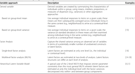
As shown in Table 1, several approaches have been used to create variables that capture collective efficacy * Correspondence:[email protected]
1Psychiatric and Neurodevelopmental Genetics Unit, Center for Human
Genetic Research, Massachusetts General Hospital, 185 Cambridge Street, Simches, Room 6.252, Boston, MA 02114, USA
Full list of author information is available at the end of the article
or related contextual-level social phenomena, such as income inequality or social capital. The most popular approach has been to create a derived variable, which entails summarizing the characteristics of individuals within a group, using means, medians, proportions, or measures of dispersion (e.g., variances) or other aggrega-tion approaches [15]. Means have been the most popular type of derived variable used in research on collective efficacy as well as other areas of multilevel research. To construct these group or contextual-level means, the major strategy has been to first average individual re-sponses to items on a given scale; these means are then subsequently averaged across individuals living in the same context (e.g., neighborhood) to arrive at a contextual-level measure [10,14,16-19].
A second approach has been to use factor analytic or latent variable models to determine whether multiple items should be grouped together in a common struct. Although factor analytic methods can be con-ducted at one or more levels of analysis (e.g., individual level, contextual level, or both), the majority of studies have focused on single-level factor analytic approaches [18]. Few studies have used latent variable approaches to study collective efficacy, even though the authors intro-ducing the concept used a hierarchical linear latent vari-able modeling approach to study collective efficacy and estimate its relationship to violent crime [9].
While both derived variables and single-level factor analytic approaches are widely used and easy to construct,
their use in multilevel research may be problematic in some cases. For example, there may be instances when more than one variable best represents the contextual-level phenomenon. Moreover, there may also be instances when it is misleading to assume the function of the items and how they relate to each other is the same at all levels of analysis. New approaches are therefore needed that allow researchers to model contextual effects using individual-level data when existing measurement strat-egies (e.g., derived variables, single-level factor analyses) are not ideal.
In an effort to expand the population health scientist’s toolkit, this paper provides an applied example of one analytic technique–multilevel factor analysis (MLFA)– that is a good alternative to existing approaches to create group or contextual-level measures. MLFA is not a new method, as it was first articulated more than 25 years ago [20-23]. However, the method has not yet been widely used, especially in population health and epidemi-ology. MLFA allows researchers to both model context-ual effects using individcontext-ual-level data without using derived variables and create variables that capture indi-vidual as well as group-level variability using one or more measures at each level of analysis (see for example [24-28]).
MLFA is part of a family of factor analytic models that seek to capture the shared variance among an observed set of variables in terms of a potentially smaller number of unobserved constructs or latent factors. Conceptually
Table 1 Approaches used to construct variables to model the effects of collective efficacy or related social-environmental variables, such as income inequality or social capital
Variable approach Description Examples
Derived variable Derived variables are created by summarizing the characteristics of individuals within a group, using means, medians, proportions, or measures of dispersion (e.g., variances) or other aggregation approaches
Based on group-level mean Use average individual responses to items on a given scale; these means are then subsequently averaged across individuals living in the same context (e.g., neighborhood) to arrive at a contextual-level measure.
[10,14,16,17]
Based on group-level variance Use average individual responses to items on a given scale; the variance (or standard deviation) in these means are then examined among individuals living in the same context (e.g., neighborhood) to arrive at a contextual-level measure.
[19]
Factor Analysis Capture the shared variance among an observed set of variables in terms of a potentially smaller number of unobserved constructs or latent factors.
Single-level factor analysis Latent factors are estimated at only one level (i.e., the individual or contextual level).
[18]
Multilevel factor analysis (MLFA) Latent factors are estimated at two-levels of analysis. Latent factors structures can differ at each level of analysis.
[24-28]
Hierarchical Latent Variable Model A special case of the 2-level MLFA that imposes stricter parameter constraints than the most general MLFA wherein latent factors are estimated at only the individual level with the factor variances decomposed into within- and between-group components.
and analytically, MLFA is distinct from the other meas-urement approaches, including derived variables, single-level factor analyses, and hierarchical latent variable models (HLVM), which all assume the constructs of interest are the same at each level of analysis. Single-level exploratory (EFA) or confirmatory factor analysis (CFA) estimates latent factors at only one level (i.e., the individual or contextual level). HLVM also estimates latent factors at only one level but captures both within- and between-level variability in those fac-tors. In contrast, MLFA allows for different latent factor structures at each level of analysis. This oc-curs because the MLFA decomposes the total sam-ple variance-covariance matrix into within-group (i.e., individual-level, within a context) and between -group (i.e., contextual-level) matrices and simultan-eously models distinct latent factor structures at each of these levels [22,29,30]. As we detail below, HLVM is a special case of MLFA. Thus, MLFA can be viewed as an analytic approach that allows the user to relax some of the potentially untenable as-sumptions and constraints imposed by the HLVM specification.
In this methodological demonstration, we apply MLFA to examine the underlying factor structure of items measuring collective efficacy and compare the results to the closest analytic alternative, the HLVM. Although our focus is on collective efficacy for demonstration pur-poses, the MLFA technique can be applied to numerous other possible contextual-level social constructs. The MLFA technique could also be extended to evaluate the measurement quality (e.g., reliability and validity) of contextual or ecological measures, including those that are directly assessed (rather than ascertained through data collected on individuals), as has been advocated by researchers concerned with“ecometrics”[6,31].
A web-based Technical Guide (see Additional file 1) is provided to guide users in implementing MLFA in MPlus. This Technical Guide is intended to guide readers on the procedures to fit and interpret results from two multilevel factor analytic models: (1) a multilevel ex-ploratory factor analysis (ML-EFA), and (2) multilevel confirmatory factor analysis (ML-CFA).
Methods
Sample and study design
Data came from the Los Angeles Family and Neighborhood Survey (L.A. FANS), a longitudinal study examining the impact of neighborhoods on children’s development and well-being [32]. The study followed a stratified random sample of 3,090 households from 65 census tracts in Los Angeles County. Within each household that contained both adults and school-aged children, a randomly selected adult (RSA) was chosen, who completed surveys at Wave
I (Spring 2000-Fall 2001). For the current study, we used data on perceptions of the neighborhood collected from the RSA. Our analytic sample consisted of 2,594 RSA respondents living in 65 census tracts. Respondents were primarily female (69.1%), Latino(a) (59.5%), and non-home owners (59.4%), with a mean age of 38.8 years (sd = 13.6).
Measures Collective efficacy
Based on previous work [9], collective efficacy was measured using 10 items that captured both perceived neighborhood informal social control and social cohe-sion [10].
Social cohesion was measured using seven items (refer to items 1–7 in Table 2) rated on a five-point scale (1 = strongly agree to 5 = strongly disagree). In-formal social control was measured using three items (refer to items 8–10 in Table 2) rated on a five-point scale (1 = very unlikely to 5 = very likely) indicating how likely the respondent would be to intervene if they witnessed these three events.
Statistical analysis
We used multilevel factor analysis (MLFA), a method that models the responses for personi in cluster j (e.g., neighborhood) to a set of M items (or indicator vari-ables), denoted yij= (y1ij,…,yMij), as a function of both
individual-level (i.e., within-group or “Level 1”) and neighborhood-level (i.e., between-group or “Level 2”) factors, represented byηWandηB, respectively.
The within-group model is given by
yij¼νjþΛWηW ijþεij; ð1Þ
where νj is a vector of the neighborhood j’s mean
responses for each of the Mitems for the population of individuals embedded in neighborhoodj; ηWijis a vector
of individual i’s values for the individual-level factors, with Ε(ηW) =0 and Var(ηW) =ψW ; ΛW is a matrix of
factor loadings describing the relationships between the individual-level factors, ηW, and the indicator variables,
yij; andεijis the residual for individualiin neighborhood
j, withΕ(ε) =0and Var(ε) =θ. Typically, with continuous ys, the residuals and factors are specified to be normally distributed, with all residuals uncorrelated with each other and with the factors.
The between-group model is given by
νj¼γþΛBηBjþζj; ð2Þ
where γis a vector of overall means for theM items; ηBjis a vector of neighborhood j’s values for the
matrix of factor loadings describing the relationships be-tween the group-level factors, ηB, and the group-level
random intercept indicators,νj; andζjis the residual for
neighborhood j, with Ε(ζ) =0 and Var(ζ) =σ. Like the within-group model, the residuals and factors are speci-fied to be normally distributed, with all residuals uncor-related with each other and with the factors.
Substituting Equation 2 into Equation 1 yields a single combined model:
yij¼γþΛWηW ijþΛBηBjþζjþεij; ð3Þ
showing that the observed responses at the individ-ual level are specified as distinct effects of both individual- and group-level factors. These effects are depicted in Figure 1 by a path diagram for a hypo-thetical six-item MLFA with two within-group and one between-group factors. The variables (observed in squares and latent in circles) within the “Individual i” box are variables that vary across each individual embedded in neighborhood j. The variables outside the “Individual i” box and within the “Neighborhood j” box vary across each neighborhood, but are con-stant for all individuals within a given neighborhood. The individual-level and neighborhood-level residuals are represented by the small arrows pointing to the observed ys and the neighborhood-level random intercept, respectively.
The model described in Equations 1 and 2 can be ex-tended to non-continuous (e.g., binary, ordinal, count, etc.) indicator variables using a generalized linear model formulation. Briefly (and as outlined in greater detail in [33,34]), any vector of indicator variables, yij, can be
expressed as the sum of the individual expected values, μijand the individual residuals,εij; that is,
yij¼μyijþεij: ð4Þ
The distribution of the residuals is chosen to corres-pond to the measurement scale of the observed indica-tors, e.g., a Bernoulli distribution for binary indicators. A link function, g, then relates the individual expected values to a linear combination of the latent factors; that is,
g μy
ij ¼νjþΛWηW ij: ð5Þ
The between-group model remains the same. In the case of continuous approximately normally distributed observed outcomes, the usual specification is the identity link function, resulting in straightforward linear regres-sions relating the observed variables to the latent factor. In the case of binary indicators, one might choose a logit link function, resulting in logistic regressions relating the observed categorical indicators to the latent factors. In the case of an observed ordinal response scale, as with our indicators of collective efficacy, we used the ordinal probit link function [35]. All models were esti-mated via weighted least squares using a diagonal weight matrix with standard errors and mean- and variance-adjusted chi-square test statistics that used a full weight matrix (WLSMV).
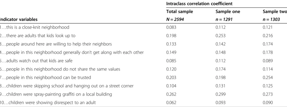
To showcase the MLFA approach, we conducted our analyses in four steps. First, we calculated intraclass cor-relation coefficients (ICCs) for each item. These ICCs
Table 2 Intraclass Correlation Coefficients (ICC) for indicator variables in the Los Angeles Family and Neighborhood Study (LAFANS) n = 2594
Intraclass correlation coefficient
Total sample Sample one Sample two
Indicator variables N = 2594 n = 1291 n = 1303
1…this is a close-knit neighborhood 0.083 0.112 0.121
2…there are adults that kids look up to 0.198 0.253 0.216
3…people around here are willing to help their neighbors 0.133 0.142 0.174
4…people in this neighborhood generally don’t get along with each other 0.149 0.148 0.178
5…adults watch out that kids are safe 0.085 0.112 0.089
6…people in this neighborhood do not share the same values 0.120 0.174 0.114
7…people in this neighborhood can be trusted 0.203 0.198 0.254
8…children were skipping school and hanging out on a street corner 0.104 0.131 0.125
9…children were spray-painting graffiti on a local building 0.262 0.299 0.273
10…children were showing disrespect to an adult 0.062 0.093 0.090
ICC refers to the proportion of variance in the indicator variable that is due to differences across neighborhoods. Neighborhoods were defined here as census tracts.
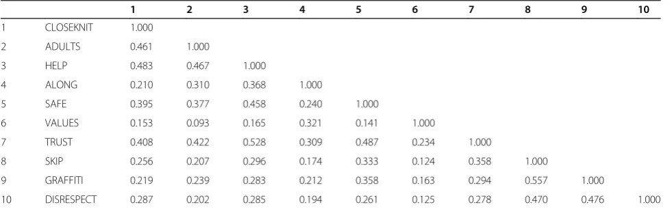
provide information about the proportion of variance in each item that is due to differences between neighbor-hoods. Second, we used polychoric correlations (where each correlation is a measure of the pairwise association for two ordinal variables, which rests upon the assump-tion of an underlying joint continuous distribuassump-tion) to examine the strength, direction, and magnitude of the associations among the items. We examined these asso-ciations in two correlation matrices: (1) the within-level (individual) matrix; and (2) the between-level (neighbor-hood) matrix. Third, we randomly split the sample into two equally sized subsamples and conducted a multilevel exploratory analysis (ML-EFA) with one subsample and a confirmatory analysis (ML-CFA) with the other. An EFA is ideal to use in situations when researchers lack
hypotheses concerning the number of latent factors underlying an item set or what the relationships are between each factor and the items; a CFA is more ap-propriate when researchers have hypotheses regarding the number of factors and the factor-item relationships or are seeking to test the validity of a theoretical model [36,37]. Both techniques are shown here for illustration purposes.
Finally, we fit the hierarchical latent variable model (HLVM) outlined by Sampson et al. [9] as a comparison. The HLVM is a special case of the MLFA, where the fac-tor measurement model is the same (i.e., same number of factors, same loading patterns, and same loading values) at the within- and between-group models and there is no between-group item-specific residual. HLMV
can also be seen as an extension of a single-level factor analysis, where the overall factor variance-covariance structure is comprised of within- and between-group variance-covariance components. The important dis-tinction between the MLFA and HLVM is that the fac-tors in the HLVM are only defined at the within-level while in the MLFA there aredistinctfactors defined at both the within- and between-level models. For the HLVM, the within-group is the same as for the MLFA, as given in Equation (1). The between-group model is given by
νj¼γþΛWηBj: ð6Þ
Substituting Equation (6) into Equation (1) yields a single combined model for the HLVM:
yij¼γþΛW ηW ijþηBj
þεij; ð7Þ
where γ is a vector of overall means for the M items; ηWijand ηBjcapture within-group across-person
variabil-ity and between-group variabilvariabil-ity, respectively, in a set of latent factors,η, withΕ(η) =0and Var(η) =ψW+ψB ; ΛW
is a matrix of factor loadings describing the relationships between the factors,η, and the indicator variables,yij; and
εijis the residual for individuali in neighborhoodj, with
Ε(ε) =0 and Var(ε) =θ. The HLVM can be more simply written as
yij¼γþΛηijþεij;
ηij¼αjþξij; ð
8Þ
showing that the observed indicators are a function of only individual-level factors with the variance-covariance of those factors explicitly decomposed by the model into within-group and between-group variance components. As with the MLFA, the HLVM can use a generalized lin-ear model approach to specify the relationships between the items and the factor in the case of non-continuous item responses. The specific HLVM model used by Sampson et al. [9], expressed as a three-level model with items nested within persons nested within clusters, imposes the additional constraints of all factor loadings being fixed at one and all item residual variances con-strained to be equal.
We conducted all analyses using Mplus software ver-sion 7. Mplus handles missing data under the missing at random assumption (MAR) using the WLSMV estima-tor, which allows missingness to be a function of the ob-served covariates, but not obob-served outcomes, as is the case for full information maximum likelihood (FIML). When there are no covariates in the model, as is the case here, this is analogous to pairwise present analysis [38,39]. Analyses also included sampling weights to adjust for non-response and the unequal probability of
selection of neighborhoods and households into the sample. Across all models, we evaluated goodness-of-fit using the model chi-square test, normed comparative fit index (CFI; [40]), root mean square error of approxima-tion (RMSEA; [41]), and the standardized root mean square residual (SRMR; [38]). These statistics provide information about how well the model-estimated popu-lation correpopu-lations reproduce the sample correpopu-lations. Acceptable model fit was determined by a non-significant chi-square test, CFI values greater than 0.95, and RMSEA and SRMR values below 0.10 [42]. The CFI, RMSEA, and SRMR values were given more emphasis than the chi-square test, as the chi-chi-square test statistic is often sig-nificant (implying there is sigsig-nificant misfit of the model to the data) when the sample size is large. In the MLFA, an SRMR is provided at both the within and between level. As there are no established guidelines for inter-preting the SRMR at the between level, we considered the guidelines that are typically applied for single-level analyses (≤0.10). We also examined the residuals for the between-level correlation matrix, which are an indicator of model fit.
Of note, there are alternative statistical software packages, such as MLwiN or MLwiN via Stata, that can be used to estimate MLFA models. Readers inter-ested in fitting the MLFA using MLwiN are referred to the MLwiN website: http://www.bristol.ac.uk/cmm/ software/mlwin/. In addition, the MLFA method can also be fit using Markov chain Monte Carlo (MCMC) methods. Such Bayesian estimation procedures may provide a particularly good alternative to maximum likelihood methods in instances when maximum likeli-hood is too computationally intensive or when there are some instances of a small number of individuals per cluster or when there are a small number of overall clusters [21].
Results
Intraclass correlation coefficients (ICC)
Correlations
As shown in Tables 3 and 4, the within level (individual) and between level (neighborhood) had different ation structures. While the average absolute correl-ation value at the within level was 0.304 (range r = 0.093 to r = 0.557), the average absolute correlation value at the between level was higher (average = 0.685; range r = 0.205 to r = 0.934). Some items also had markedly differently correlations at each level. For example, the items“people here do not get along with each other”and“people would intervene if children were spray painting graffiti” had a very strong correlation at the between-level (r = 0.858), but a weak correlation at the within-level (r = 0.239). These finding suggest the item-to-item relationships differ across the two levels of analysis (within- and between-level).
Multilevel factor analysis (MLFA) results Multilevel exploratory factor analysis (ML-EFA)
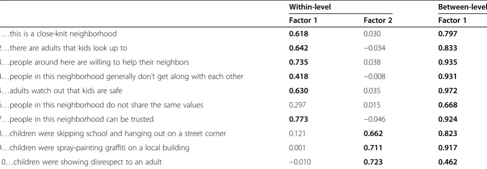
The final ML-EFA model, which was selected based on good model-data consistency, parsimony, and interpret-ability, had two within-level factors and one between-level factor (Table 5). In this factor solution, the largest factor loadings for each item at the within level (0.418 to 0.773) and between level (0.462 to 0.972) ranged from moderate to high. In addition to good overall model fit, as evidenced by the CFI of 0.947 and RMSEA of 0.059, this solution also had excellent model fit specifically at the within and between levels, as shown in the SRMR values at each level 0.039 and 0.068, respectively. In con-trast, the next best fitting model–the two factor within and two-factor between model – had a good overall fit (SRMRwithin= 0.039; SRMRbetween= 0.045). However, the second between-level factor had only one significantly
loading item (refer to page 21 of the online Technical Guide.
Beyond its empirical fit, the ML-EFA solution was also aligned with prior theory. At the within level, the first factor mapped on to the construct social cohesion and the second factor mapped on to the construct informal social control, as described by others [9,10]. At the be-tween level, the indicator variables only supported one overarching factor, which has previously been labeled as collective efficacy [9,10]. Interestingly, the sixth item (people in this neighborhood do not share the same values) did not load significantly on either factor at the within level, but had a significant factor loading at the be-tween level. This finding illustrates that indicator variables can perform differently at each level of analysis and there-fore items should only be removed from a MLFA if they are determined not to function at both levels of analysis.
The first and second within-level factors were moder-ately correlated (r = 0.521). The communalities, or item-specific R2 values, which refer to the proportion of an indicator’s total variance accounted for by the factor solution, ranged at the within level from a low of 8.4% (for respondents’ rating of people in the neighborhood sharing the same values) to a high of 57.1% (for respon-dents’rating of people’s willingness to help neighbors) at the within level. At the between level, the communalities were higher across the items, ranging from a low of 21.4% (for neighborhoods’ collective tendency to inter-vene if children show disrespect to an adult) to a high of 94.4% (for neighborhoods’collective tendency to watch out that kids are safe).
Multilevel confirmatory factor analysis (ML-CFA)
The ML-EFA results from the first subsample were cross-validated using ML-CFA for the second subsample.
Table 3 Correlations among indicators at the within-level
1 2 3 4 5 6 7 8 9 10
1 CLOSEKNIT 1.000
2 ADULTS 0.461 1.000
3 HELP 0.483 0.467 1.000
4 ALONG 0.210 0.310 0.368 1.000
5 SAFE 0.395 0.377 0.458 0.240 1.000
6 VALUES 0.153 0.093 0.165 0.321 0.141 1.000
7 TRUST 0.408 0.422 0.528 0.309 0.487 0.234 1.000
8 SKIP 0.256 0.207 0.296 0.174 0.333 0.124 0.358 1.000
9 GRAFFITI 0.219 0.239 0.283 0.212 0.358 0.163 0.294 0.557 1.000
10 DISRESPECT 0.287 0.202 0.285 0.194 0.261 0.125 0.278 0.470 0.476 1.000
CLOSEKNIT = this is a close-knit neighborhood; ADULTS = there are adults that kids look up to; HELP = people here are willing to help their neighbors; ALONG = people here don’t get along with each other; SAFE = adults watch out that kids are safe; VALUES = people here do not share the same values; TRUST = people in this neighborhood can be trusted; SKIP = people would intervene if children were skipping school and hanging out on the corner; GRAFFITI = people would intervene if children were spray-painting graffiti; DISRESPECT = people would intervene if children were showing disrespect to an adult. Items 4 and 6 were reverse coded.
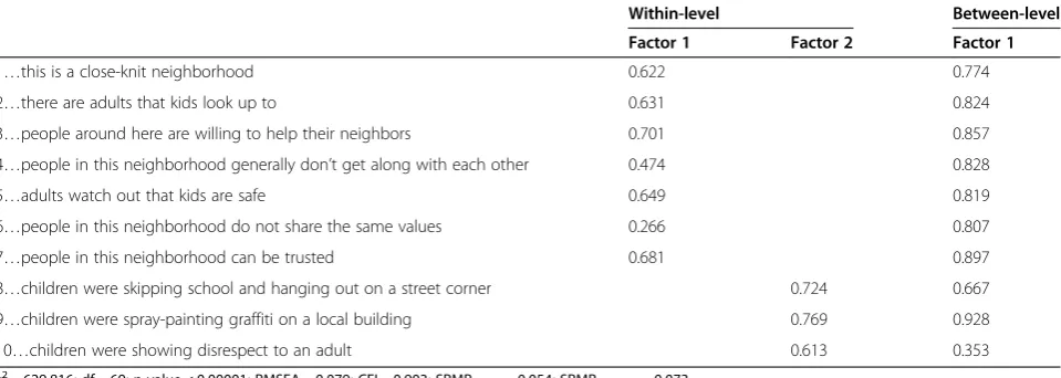
As shown in Table 6, the fit of the ML-CFA model was good (CFI = 0.903; RMSEA = 0.079; SRMRwithin= 0.054; SRMRbetween= 0.073). By and large, factor loadings in the ML-CFA were similar to the ML-EFA.
We also ran an alternative ML-CFA specification with the constraints imposed by the Sampson et al. version of the HLVM described earlier. The overall fit of this model was markedly worse than the ML-CFA without these restrictions (χ2= 1445.265; df = 86; p-value < 0.001; RMSEA = 0.110; CFI = 0.766; SRMRwithin= 0.095; SRMRbetween= 0.325), suggesting that a more restricted model lacked the model-data consistency observed with the less restrictive ML-CFA. Of note, a single-level fac-tor analysis, which is the equivalent of adding to the HLVM a further constraint of zero between-level factor variance, would have a poorer fit than the HLVM. Al-though not the case here, it is possible that for another
dataset, the HLVM specification could fit equivalent to the MLFA. Such a finding would suggest that the data do not support a different factor structure at the within and between-group levels, and the HLVM could be favored as a more parsimonious model. A researcher, however, would not be able to make this determination without comparing the HLVM to the MLFA.
Discussion
This methodological demonstration of MLFA to collect-ive efficacy shows that use of either simple aggregation methods, in the form of derived variables, or single-level factor analyses, may not be the best way to construct contextual-level variables from individual-level data. We arrived at this conclusion based on three sets of results. First, we found that ICC values were not the same for every item; some items showed quite high
neighborhood-Table 5 Factor loadings of indicators for the multi-level exploratory factor analysis (ML-EFA)
Within-level Between-level
Factor 1 Factor 2 Factor 1
1…this is a close-knit neighborhood 0.618 0.030 0.797
2…there are adults that kids look up to 0.642 −0.034 0.833
3…people around here are willing to help their neighbors 0.735 0.038 0.935
4…people in this neighborhood generally don’t get along with each other 0.418 −0.008 0.931
5…adults watch out that kids are safe 0.630 0.035 0.972
6…people in this neighborhood do not share the same values 0.297 0.015 0.668
7…people in this neighborhood can be trusted 0.773 −0.046 0.924
8…children were skipping school and hanging out on a street corner 0.121 0.662 0.823
9…children were spray-painting graffiti on a local building 0.001 0.711 0.917
10…children were showing disrespect to an adult −0.010 0.723 0.462
χ2
= 337.222; df = 61; p-value < 0.00001; CFI = 0.947; RMSEA = 0.059; SRMRwithin = 0.039; SRMRbetween = 0.068. All factor loadings in an EFA are standardized.High EFA loadings appear in bold.
Items 4 and 6 were reverse coded.
Table 4 Correlations among indicators at the between-level
1 2 3 4 5 6 7 8 9 10
1 CLOSEKNIT 1.000
2 ADULTS 0.735 1.000
3 HELP 0.773 0.862 1.000
4 ALONG 0.593 0.758 0.855 1.000
5 SAFE 0.749 0.853 0.897 0.902 1.000
6 VALUES 0.561 0.620 0.668 0.754 0.705 1.000
7 TRUST 0.742 0.842 0.870 0.834 0.934 0.653 1.000
8 SKIP 0.826 0.641 0.731 0.677 0.765 0.650 0.697 1.000
9 GRAFFITI 0.729 0.858 0.870 0.857 0.865 0.725 0.823 0.757 1.000
10 DISRESPECT 0.489 0.205 0.478 0.316 0.254 0.257 0.320 0.480 0.382 1.000
level variation and others showed very little. The lack of uniformity in between-neighborhood variation across these items suggests neighborhood context may have dif-fering levels of salience across this set of items and that not all items should be treated equally in terms of their importance to understanding neighborhoods.
Second, the correlation structure of the items was dif-ferent across the individual (within) and neighborhood (between) levels. Specifically, the correlation among items was much higher at the between level than the within. Moreover, how the items related to each other also differed across levels; some items had high correla-tions at one level and modest correlacorrela-tions at the other. These findings provided an initial sign that there may be different factor structures at the two levels of analysis.
Third, when we ran the MLFA, we found that the best-fitting model was one that modeled collective effi-cacy as a two dimensional construct at the within level, consisting of the two latent constructs informal social control and social cohesion, and a one dimensional construct at the between level, consisting of collective efficacy. This two-factor within and one-factor between model was confirmed in the ML-CFA. Imposing an identical factor structure at both levels resulted in a worse-fitting model, particularly when we imposed a set of stricter constraints described in the original paper introducing collective efficacy [9]. While the stricter constraints may be reasonable and could be supported by the data in some cases, there may be instances, such as the case here, where the items were not all equally good indicators of collective efficacy and thus imposing equal factor loadings and equal residual variances con-straints was not consistent with the observed data. We also found that the items performed differently in terms of their factor loadings at the within compared to between level. For example, the item “people in this
neighborhood do not share the same values” did not load at the within level, but loaded at the between. Taken together, the results of the current study suggest that collective efficacy, and perhaps other social con-structs, can have very different meanings at each level of analysis and are perhaps most appropriately studied at the neighborhood level as one overarching construct and not divided into its two dimensions, informal social control and social cohesion, as has been done in some prior studies (see for example [13,43]).
Our study has the following limitations. The measure of collective efficacy was not identical to the original measure [9]. It is possible our results would have been different had we used a different measure of collective efficacy. The number of neighborhoods in this study (n = 65) was also small relative to other studies. More-over, our definition of neighborhoods was based on an administrative definition (i.e., Census tract), which may not adequately reflect meaningful geographic boundaries that represent distinct social experiences or cultures [44,45]. Though an imperfect measure to define neighbor-hoods, Census tracts are most commonly used in multi-level research in the United States [8].
Finally, the MLFA technique is, of course, not without its limitations. For example, it can be computationally intensive. Most software also only allow for two-level structures. In spite of these challenges, results of our analysis underscore the potential utility of MLFA and suggest that using other more easily implemented ap-proaches, such as single-level factor analyses, may not be ideal. As we showed, the MFLA method revealed dif-ferent latent factor structures at each level of analysis. Our results also demonstrated that imposing a simpler factor structure, with identical factor structures at each level, was not consistent with the data and resulted in a poorer-fitting model.
Table 6 Standardized factor loadings of items for the Multi-Level Confirmatory Factor Analysis (ML-CFA)
Within-level Between-level
Factor 1 Factor 2 Factor 1
1…this is a close-knit neighborhood 0.622 0.774
2…there are adults that kids look up to 0.631 0.824
3…people around here are willing to help their neighbors 0.701 0.857
4…people in this neighborhood generally don’t get along with each other 0.474 0.828
5…adults watch out that kids are safe 0.649 0.819
6…people in this neighborhood do not share the same values 0.266 0.807
7…people in this neighborhood can be trusted 0.681 0.897
8…children were skipping school and hanging out on a street corner 0.724 0.667
9…children were spray-painting graffiti on a local building 0.769 0.928
10…children were showing disrespect to an adult 0.613 0.353
χ2
= 629.816; df = 69; p-value < 0.00001; RMSEA = 0.079; CFI = 0.903; SRMRwithin= 0.054; SRMRbetween= 0.073.
Results of this study have several important implica-tions for measuring social environments potentially linked to health. Multilevel researchers have lamented the lack of progress in identifying novel measurement tools to characterize contextual-level constructs and as a result have called for new approaches [3-8]. Although more work is needed, results of the current study suggest that MLFA may be a promising method to con-struct variables from individual-level data for use in multilevel analyses. The MLFA technique allows re-searchers to use individual-level items to construct mea-sures of the social context using a more flexible approach than other types of hierarchical models. The MLFA approach can also be easily applied with survey data, which remains the most common and cost effective type of data collected. Moreover by using MLFA, re-searchers establish the measurement model necessary for estimating a multilevel structural equation model (ML-SEM), where direct and indirect effects between latent variables, covariates, and individual items, existing at two or more levels of analysis, are examined [42,46,47]. Although still not widely used in epidemiology or popula-tion health, SEM models are an alternative to tradipopula-tional techniques that can be used for exploratory or hypothesis-generating purposes [48] or to test more complex rela-tionships between a set of variables [49,50].
In conclusion, our results suggest MLFA is a promis-ing alternative to uspromis-ing derived variables and spromis-ingle-level factor analytic approaches. Future studies are warranted to validate the current results in relation to collective efficacy and extend the MLFA technique to other di-mensions of the neighborhood environment as well as other social contexts that influence health.
Additional file
Additional file 1:Technical Appendix for the article: Modeling contextual effects using individual-level data and without aggregation: an illustration of multilevel factor analysis (MLFA) with collective efficacy.
Competing interests
The authors declare that they have no competing interests.
Authors’contributions
ECD conceptualized the analytic plan, oversaw the analysis, interpreted results, drafted the manuscript, and approved the final version. KEM helped Dr. Dunn conceptualize the original study design, met regularly to review results, reviewed and edited the early draft of the manuscript, and approved the final version. WRJ carried out the analyses, helped with interpretation of results, edited the early manuscripts, and approved the final version. SVS worked with Dr. Dunn to conceptualize the original study design, reviewed and aided in interpreting early results, and approved the final version. All authors read and approved the final manuscript.
Author details
1Psychiatric and Neurodevelopmental Genetics Unit, Center for Human
Genetic Research, Massachusetts General Hospital, 185 Cambridge Street, Simches, Room 6.252, Boston, MA 02114, USA.2Division of Epidemiology and
Biostatistics, School of Public Health, Georgia State University, Atlanta, GA 30302, USA.3Harvard Graduate School of Education, 6 Appian Way, Cambridge, MA 02138, USA.4Department of Social and Behavioral Sciences,
Harvard T.H. Chan School of Public Health, 677 Huntington Avenue, Kresge Building 7th Floor, 716, Boston, Massachusetts 02115, USA.
Received: 21 July 2014 Accepted: 28 March 2015
References
1. Pickett KE, Pearl M. Multilevel analyses of neighbourhood socioeconomic context and health outcomes: a critical review. J Epidemiol Community Health. 2001;55:111–22.
2. Mair CF, Diez Roux AV, Galea S. Are neighborhood characteristics associated with depressive symptoms? A critical review. J Epidemiol Community Health. 2008;62(11):940–6.
3. Diez Roux AV, Auchincloss AH. Understanding the social determinants of behaviours: can new methods help? Int J Drug Policy. 2009;20:227–9. 4. Messer LC. Invited commentary: beyond the metrics for measuring
neighborhood effects. Am J Epidemiol. 2007;165(8):868–71.
5. Diez Roux AV. Next steps in understanding the multilevel determinants of health. J Epidemiol Community Health. 2008;62:957–9.
6. Raudenbush SW, Sampson RJ. Ecometrics: toward a science of assessing ecological settings, with application to the systematic social observation of neighborhoods. Sociol Methodol. 1999;29:1–41.
7. Mujahid MS, Diez Roux AV, Morenoff JD, Raghunathan T. Assessing the measurement properties of neighborhood scales: from psychometrics to ecometrics. Am J Epidemiol. 2007;165(8):858–67.
8. Dunn EC, Masyn KE, Yudron M, Jones SM, Subramanian SV. Translating multilevel theory into multilevel research: challenge and opportunities for understanding the social determinants of psychiatric disorders. Soc Psychiatry Psychiatr Epidemiol. 2014;49:859–72.
9. Sampson RJ, Raudenbush S, Earls F. Neighborhoods and violent crime: a multilevel study of collective efficacy. Science. 1997;277:918–24. 10. Cohen DA, Finch BK, Bower A, Sastry N. Collective efficacy and obesity: the
potential influence of social factors on health. Soc Sci Med. 2006;62:769–78. 11. Sampson RJ. Great american city: Chicago and the enduring neighborhood
effect. Chicago, IL: University of Chicago Press; 2012.
12. Sampson RJ, Morenoff JD, Earls F. Beyond social capital: spatial dynamics of collective efficacy for children. Am Sociol Rev. 1999;64:633–60.
13. Sampson RJ. Collective efficacy theory: Lessons learned and directions for future inquiry. In: Cullen FT, Wright JP, Blevins KR, editors. Taking stock: The status of criminological Theory, vol. 15. New Brunswick, NJ: Transaction Publishers; 2008. p. 149–66.
14. Ahern J, Galea S. Collective efficacy and major depression in urban neighborhoods. Am J Epidemiol. 2011;173(12):1453–62.
15. Diez Roux AV. A glossary for multilevel analysis. J Epidemiol Community Health. 2002;56:588–94.
16. Xue Y, Leventhal T, Brooks-Gunn J, Earls FJ. Neighborhood residence and mental health problems of 5- to 11-year olds. Arch Gen Psychiatry. 2005;62:554–63.
17. Kim J. Influence of neighbourhood collective efficacy on adolescent sexual behaviour: variation by gender and activity participation. Child Care Health Dev. 2010;36(5):646–54.
18. Cagney KA, Glass TA, Skarupski KA, Barnes LL, Schwartz BS, Mendes de Leon CF. Neighborhood-level cohesion and disorder: measurement and validation in two older adult urban populations. J Gerontol B Psychol Sci Soc Sci. 2009;64(3):415–24.
19. De Maio FG. Income inequality measures. J Epidemiol Community Health. 2007;61:849–52.
20. Longford N, Muthen BO. Factor analysis for clustered observations. Psychometrika. 1992;57:581–97.
21. Goldstein H, Browne W. Multilevel factor analysis modelling using Markov Chain Monte Carlo (MCMC) estimation. In: Marcoulides GA, Moustaki M, editors. Latent variable and latent structure models. Mahwah, NJ: Lawrence Erlbaum Associates Inc Publishers; 2002. p. 225–44.
22. Muthén BO. Multilevel factor analysis of class and student achievement components. J Educ Meas. 1991;28(4):338–54.
24. Toland MD, De Ayala RJ. A multilevel factor analysis of students’evaluations of teaching. Educ Psychol Meas. 2005;65(2):272–96.
25. Reise SP, Ventura J, Neuchterlein KH, Kim KH. An illustration of multilevel factor analysis. J Pers Assess. 2005;84(2):126–36.
26. Dyer NG, Hanges PJ, Hall RJ. Applying multilevel confirmatory factor analysis techniques to the study of leadership. Leadersh Q. 2005;16:149–67. 27. Dedrick RF, Greenbaum PE. Multilevel confirmatory factor analysis of a scale
measuring interagency collaboration of children’s mental health agencies. J Emot Behav Disord. 2011;19:27–40.
28. Dunn EC, Masyn KE, Jones SM, Subramanian SV, Koenen KC. Measuring psychosocial climates using individual responses: An application of multilevel factor analysis to examining students in schools. Prev Sci. In press. 29. Muthén BO. Multilevel covariance structure analysis. Sociol Methods Res.
1994;22:376–98.
30. Hox JJ. Multilevel analysis: Techniques and applications. 2nd ed. New York, NY: Routledge; 2010.
31. Raudenbush SW. The quantitative assessment of neighborhood social environments. In: Kawachi I, Berkman LF, editors. Neighborhoods and health. New York, NY: Oxford University Press; 2003. p. 112–31.
32. Sastry N, Ghosh-Dastidar B, Adams J, Pebley AR. The design of a multilevel survey of children, families, and communities: the Los Angeles Family and Neighborhood Survey. Soc Sci Res. 2006;35(4):1000–24.
33. McCullagh P, Nelder JA. Generalized linear models. 2nd ed. Boca Raton, Florida: Chapman & Hall/CRC; 1989.
34. Skrondal A, Rabe-Hesketh S. Generalized latent variable modeling: Multilevel, longitudinal, and structural equation models. Boca Raton, Florida: Chapman & Hall/CRC; 2004.
35. Flora DB, Curran PJ. An empirical evaluation of alternative methods of estimation for confirmatory factor analysis with ordinal data. Psychol Methods. 2004;9(4):466–91.
36. Brown TA. Confirmatory factor analysis for applied research. New York, NY: Guilford Press; 2006.
37. Kline P. An easy guide to factor analysis. London, England: Routledge; 1994. 38. Muthén LK, Muthén BO. Mplus user’s guide. Los Angeles, CA: Muthén &
Muthén; 1998. 1998–2010.
39. Asparouhov T, Muthén B. Weighted least squares estimation with missing data. 2010; Available from: http://www.statmodel.com/download/ GstrucMissingRevision.pdf.
40. Bentler PM. Comparative fit indexes in structural models. Psychol Bull. 1990;107:238–46.
41. Steiger JH. Structural model evaluation and modification: an interval estimation approach. Multivar Behav Res. 1990;25:173–80.
42. Kline RB. Principles and practice of structural equation modeling. 3rd ed. New York, NY: Guilford Press; 2010.
43. Silver E, Miller LL. Sources of informal social control in chicago neighborhoods’. Criminology. 2004;42(3):551–83.
44. Merlo J. Invited commentary: multilevel analysis of individual heterogeneity-a fundheterogeneity-amentheterogeneity-al critique of the current probheterogeneity-abilistic risk fheterogeneity-actor epidemiology. Am J Epidemiol. 2014;180(2):208–12. discussion 213–4.
45. Merlo J. Invited commentary: multilevel analysis of individual heterogeneity-a fundheterogeneity-amentheterogeneity-al critique of the current probheterogeneity-abilistic risk fheterogeneity-actor epidemiology. Am J Epidemiol. 2014;80(2):208-12. Discussion 213-204. doi:10.1093/aje/ kwu108.
46. Marsh HW, Ludtke O, Robitzsch A, Trautwein U, Asparouhov T, Muthen B, et al. Doubly-latent models of school contextual effects: integrating multilevel and structural equation approaches to control measurement and sampling error. Multivar Behav Res. 2009;44:764–802.
47. MacCallum RC, Austin JT. Applications of structural equation modeling in psychological research. Annu Rev Psychol. 2000;51:201–26.
48. VanderWeele TJ. Invited commentary: structural equation models and epidemiologic analysis. Am J Epidemiol. 2012;176(7):608–12.
49. Arlinghaus A, Lombardi DA, Willetts JL, Folkard S, Christiani DC. A structural equation modeling approach to fatigue-related risk factors for occupational injury. Am J Epidemiol. 2012;176(7):597–607.
50. Factor-Litvak P, Sher A. Invited commentary: coming out of the box. Am J Epidemiol. 2009;169(10):1179–81.
51. Browning CR, Cagney KA. Neighborhood structural disadvantage, collective efficacy, and self-rated physical health in urban settings. J Health Soc Behav. 2002;43:383–99.
Submit your next manuscript to BioMed Central and take full advantage of:
• Convenient online submission
• Thorough peer review
• No space constraints or color figure charges
• Immediate publication on acceptance
• Inclusion in PubMed, CAS, Scopus and Google Scholar
• Research which is freely available for redistribution