A comprehensive survey on machine learning for networking: evolution, applications and research opportunities

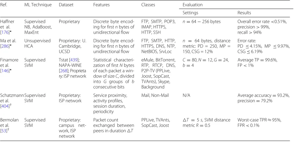
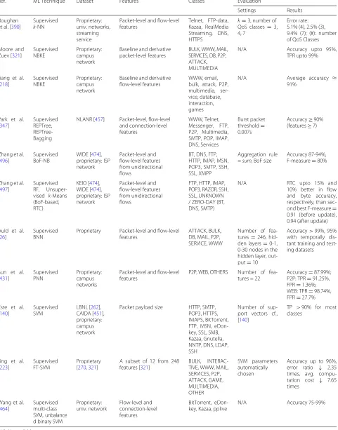
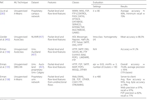
R E S E A R C H

Open Access

A comprehensive survey on machine

learning for networking: evolution,

applications and research opportunities

Raouf Boutaba

, Mohammad A. Salahuddin

, Noura Limam

, Sara Ayoubi

, Nashid Shahriar

,

Felipe Estrada-Solano

and Oscar M. Caicedo

Abstract

Machine Learning (ML) has been enjoying an unprecedented surge in applications that solve problems and enable automation in diverse domains. Primarily, this is due to the explosion in the availability of data, significant

improvements in ML techniques, and advancement in computing capabilities. Undoubtedly, ML has been applied to various mundane and complex problems arising in network operation and management. There are various surveys on ML for specific areas in networking or for specific network technologies. This survey is original, since it jointly presents the application of diverse ML techniques in various key areas of networking across different network technologies. In this way, readers will benefit from a comprehensive discussion on the different learning paradigms and ML

techniques applied to fundamental problems in networking, including traffic prediction, routing and classification, congestion control, resource and fault management, QoS and QoE management, and network security. Furthermore, this survey delineates the limitations, give insights, research challenges and future opportunities to advance ML in networking. Therefore, this is a timely contribution of the implications of ML for networking, that is pushing the barriers of autonomic network operation and management.

Keywords: Machine learning, Traffic prediction, Traffic classification, Traffic routing, Congestion control, Resource management, Fault management, QoS and QoE management, Network security

1 Introduction

Machine learning (ML) enables a system to scrutinize data and deduce knowledge. It goes beyond simply learning or extracting knowledge, to utilizing and improving knowl-edge over time and with experience. In essence, the goal of ML is to identify and exploit hidden patterns in “training” data. The patterns learnt are used to analyze unknown data, such that it can be grouped together or mapped to the known groups. This instigates a shift in the traditional programming paradigm, where programs are written to automate tasks. MLcreatesthe program (i.e.model) that fits the data. Recently, ML is enjoying renewed interest. Early ML techniques were rigid and incapable of tolerating any variations from the training data [134].

*Correspondence:[email protected]

1_{David R. Cheriton School of Computer Science, University of Waterloo,}

Waterloo, Canada

Full list of author information is available at the end of the article

Recent advances in ML have made these techniques flexible and resilient in their applicability to various real-world scenarios, ranging from extraordinary to mundane. For instance, ML in health care has greatly improved the areas of medical imaging and computer-aided diag-nosis. Ordinarily, we often use technological tools that are founded upon ML. For example, search engines extensively use ML for non-trivial tasks, such as query suggestions, spell correction, web indexing and page rank-ing. Evidently, as we look forward to automating more aspects of our lives, ranging from home automation to autonomous vehicles, ML techniques will become an increasingly important facet in various systems that aid in decision making, analysis, and automation.

Apart from the advances in ML techniques, various other factors contribute to its revival. Most importantly, the success of ML techniques relies heavily on data [77]. Undoubtedly, there is a colossal amount of data in todays’ networks, which is bound to grow further with emerging

© The Author(s). 2018Open AccessThis article is distributed under the terms of the Creative Commons Attribution 4.0

International License (http://creativecommons.org/licenses/by/4.0/), which permits unrestricted use, distribution, and

networks, such as the Internet of Things (IoT) and its billions of connected devices [162]. This encourages the application of ML that not only identifies hidden and unexpected patterns, but can also be applied to learn and understand the processes that generate the data.

Recent advances in computing offer storage and pro-cessing capabilities required for training and testing ML models for the voluminous data. For instance, Cloud Computing offers seemingly infinite compute and storage resources, while Graphics Processing Units [342] (GPUs) and Tensor Processing Units [170] (TPUs) provide accel-erated training and inference for voluminous data. It is important to note that a trained ML model can be deployed for inference on less capable devices e.g. smartphones. Despite these advances, network opera-tions and management still remains cumbersome, and network faults are prevalent primarily due to human error [291]. Network faults lead to financial liability and defamation in reputation of network providers. There-fore, there is immense interest in building autonomic (i.e. configuring, healing, optimizing and self-protecting) networks [28] that are highly resilient.

Though, there is a dire need for cognitive control in net-work operation and management [28], it poses a unique set of challenges for ML. First, each network is unique and there is a lack of enforcement of standards to attain uniformity across networks. For instance, the enterprise network from one organization is diverse and disparate from another. Therefore, the patterns proven to work in one network may not be feasible for another network of the same kind. Second, the network is continually evolving and the dynamics inhibit the application of a fixed set of patterns that aid in network operation and management. It is almost impossible to manually keep up with network administration, due to the continuous growth in the num-ber of applications running in the network and the kinds of devices connected to the network.

Key technological advances in networking, such as net-work programmability via Software-Defined Netnet-working (SDN), promote the applicability of ML in networking. Though, ML has been extensively applied to problems in pattern recognition, speech synthesis, and outlier detec-tion, its successful deployment for network operations and management has been limited. The main obstacles include what data can be collected from and what control actions can be exercised on legacy network devices. The ability to program the network by leveraging SDN alleviates these obstacles. The cognition from ML can be used to aid in the automation of network operation and management tasks. Therefore, it is exciting and non-trivial to apply ML techniques for such diverse and complex problems in networking. This makes ML in networking an interesting research area, and requires an understanding of the ML techniques and the problems in networking.

In this paper, we discuss the advances made in the application of ML in networking. We focus on traffic engi-neering, performance optimization and network security. In traffic engineering, we discuss traffic prediction, clas-sification and routing that are fundamental in providing differentiated and prioritized services. In performance optimization, we discuss application of ML techniques in the context of congestion control, QoS/QoE correlation, and resource and fault management. Undoubtedly, secu-rity is a cornerstone in networking and in this regard, we highlight existing efforts that use ML techniques for network security.

The primary objective of this survey is to provide a comprehensive body of knowledge on ML techniques in support of networking. Furthermore, we complement the discussion with key insights into the techniques employed, their benefits, limitations and their feasibility to real-world networking scenarios. Our contributions are summarized as follows:

– A comprehensive view of ML techniques in

network-ing. We review literature published in peer-reviewed venues over the past two decades that have high impact and have been well received by peers. The works selected and discussed in this survey are com-prehensive in the advances made for networking. The key criteria used in the selection is a combination of the year of publication, citation count and merit. For

example, consider two papers A and B published in

the same year with citation counts x and y,

respec-tively. Ifx is significantly larger than y, A would be

selected for discussion. However, upon evaluatingB,

if it is evidenced that it presents original ideas, criti-cal insights or lessons learnt, then it is also selected for discussion due to its merit, despite the lower citation count.

– A purposeful discussion on the feasibility of the ML

techniques for networking. We explore ML tech-niques in networking, including their benefits and limitations. It is important to realize that our coverage of networking aspects are not limited to a specific net-work technology (e.g. cellular netnet-work, wireless sensor network (WSN), mobile ad hoc network (MANET), cognitive radio network (CRN)). This gives readers a broad view of the possible solutions to networking problems across network technologies.

– Identification of key challenges and future research

Though there are various surveys on ML in network-ing [18,61,82,142,246,339], this survey is purposefully different. Primarily, this is due to its timeliness, the com-prehensiveness of ML techniques covered, and the vari-ous aspects of networking discussed, irrespective of the network technology. For instance, Nguyen and Armitage [339], though impactful, is now dated and only addresses traffic classification in networking. Whereas, Fadlullah et al. [142] and Buczak et al. [82], both state-of-the-art surveys, have a specialized treatment of ML to spe-cific problems in networking. On the other hand, Klaine et al. [246], Bkassiny et al. [61] and Alsheikh et al. [18], though comprehensive in their coverage of ML techniques in networking, are specialized to specific network tech-nology i.e. cellular network, CRN and WSN, respectively. Therefore, our survey provides a holistic view of the appli-cability, challenges and limitations of ML techniques in networking.

We organize the remainder of this paper as follows.

In Section 2, we provide a primer on ML, which

dis-cusses different categories of ML-based techniques, their essential constituents and their evolution. Sections3, 4

and 5 discuss the application of the various ML-based

techniques for traffic prediction, classification and rout-ing, respectively. We present the ML-based advances in performance management, with respect to congestion control, resource management, fault management, and QoS/QoE management for networking in Sections 6,7,8

and9. In Section10, we examine the benefits of ML for anomaly and misuse detection for intrusion detection in networking. Finally, we delineate the lessons learned, and future research challenges and opportunities for ML in networking in Section11. We conclude in Section12with a brief overview of our contributions. To facilitate reading, Fig.1presents a conceptual map of the survey, and Table1

provides the list of acronyms and definitions for ML.

2 Machine learning for networking—a primer In 1959, Arthur Samuel coined the term “Machine Learn-ing”, as“the field of study that gives computers the ability to learn without being explicitly programmed”[369]. There are four broad categories of problems that can leverage ML, namely,clustering,classification,regressionandrule extraction [79]. In clustering problems, the objective is to group similar data together, while increasing the gap between the groups. Whereas, in classification and regres-sion problems, the goal is to map a set of new input data to a set of discrete or continuous valued output, respectively. Rule extraction problems are intrinsically different, where the goal is to identify statistical relationships in data.

ML techniques have been applied to various problem domains. A closely related domain consists of data anal-ysis for large databases, called data mining [16]. Though, ML techniques can be applied to aid in data mining, the

goal of data mining problems is to critically and metic-ulously analyze data—its features, variables, invariants, temporal granularity, probability distributions and their transformations. However, ML goes beyond data mining to predict future events or sequence of events.

Generally, ML is ideal for inferring solutions to prob-lems that have a large representative dataset. In this way, as illustrated in Fig. 2, ML techniques are designed to identify and exploit hidden patterns in data for (i) describ-ing the outcome as a groupdescrib-ing of data for clusterdescrib-ing problems, (ii) predicting the outcome of future events for classification and regression problems, and (iii) evaluat-ing the outcome of a sequence of data points for rule extraction problems. Though, the figure illustrates data and outcome in a two-dimensional plane, the discus-sion holds for multi-dimendiscus-sional datasets and outcome functions. For instance, in the case of clustering, the out-come can be a non-linear function in a hyperplane that discriminates between groups of data. Networking prob-lems can be formulated as one of these probprob-lems that can leverage ML. For example, a classification problem in networking can be formulated to predict the kind of secu-rity attack: Denial-of-Service (DoS), User-to-Root (U2R), Root-to-Local (R2L), or probing, given network condi-tions. Whereas, a regression problem can be formulated to predict of when a future failure will transpire.

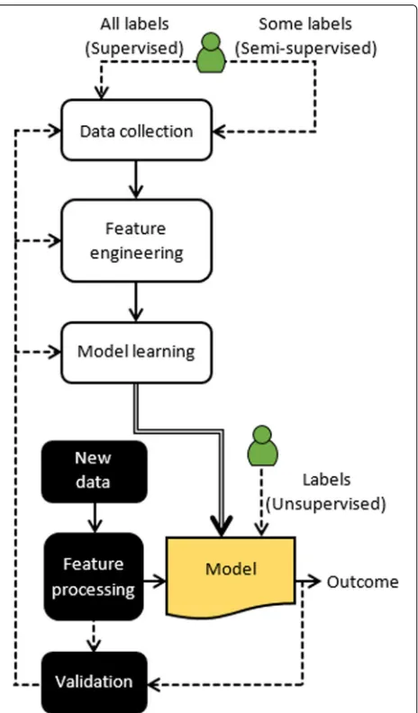
Though there are different categories of problems that enjoy the benefits of ML, there is a generic approach to building ML-based solutions. Figure 3 illustrates the key constituents in designing ML-based solutions for net-working.Data collectionpertains to gathering, generating and, or defining the set of data and the set of classes of interest.Feature engineeringis used to reduce dimen-sionality in data and identify discriminating features that reduce computational overhead and increase accuracy. Finally, ML techniques carefully analyze the complex inter- and intra-relationships in data and learn a model for the outcome.

For instance, consider an example of Gold values over time, as illustrated in Fig.2c. Naïvely, a linear regression model, shown as a best-fit line through the historical data, can facilitate in predicting future values of Gold. There-fore, once the ML model is built, it can be deployed to deduce outcomes from new data. However, the outcomes are periodically validated, since they can drift over time, known as concept drifting. This can be used as an indi-cator for incremental learning and re-training of the ML model. In the following subsections, we discuss each of the components in Fig.3.

2.1 Learning paradigms

There are four learning paradigms in ML, supervised,

Fig. 1Conceptual map of the survey

engineering, and establishing ground truth. Recall, the objective is to infer an outcome, given some dataset. The dataset used in constructing the ML model is often denoted as training data and labels are associ-ated with training data if the user is aware of the description of the data. The outcome is often per-ceived as the identification of membership to a class of interest.

There are two schools of thought on the methodol-ogy for learning;generativeanddiscriminative[333]. The basis for the learning methodologies is rooted in the famous Bayes’ theorem for conditional probability and

the fundamental rule that relates joint probability to con-ditional probability. Bayes’ theorem is stated as follows. Given two eventsAandB, the conditional probability is defined as

P(A|B)= P(B|A)×P(A)

P(B) ,

which is also stated as

posterior= likelihood×prior

Table 1List of acronyms for machine learning

AdaBoost Adaptive Boosting

AIWPSO Adaptive Inertia Weight Particle Swarm Optimization

BN Bayesian Network

BNN Bayesian Neural Network

BP BackPropagation

CALA Continuous Action-set Learning Automata

CART Classification and Regression Tree

CMAC Cerebellar Model Articulation Controller

DBN Deep belief Network

DBSCAN Density-based Spatial Clustering of Applications with Noise

DE Differential Evolution

DL Deep Learning

DNN Deep Neural Network

DQN Deep Q-Network

DT Decision Tree

EM Expectation Maximization

EMD Entropy Minimization Discretization

FALA Finite Action-set Learning Automata

FCM Fuzzy C Means

FNN Feedforward Neural Network

GD Gradient Descent

HCA Hierarchical Clustering Analysis

HMM Hidden Markov Model

HNN Hopfield Neural Network

ID3 Iterative Dichotomiser 3

k-NN k-Nearest Neighbor KDE Kernel Density Estimation

LDA Linear Discriminant Analysis

LSTM Long Short-term Memory

LVQ Learning Vector Quantization

MART Multiple Additive Regression Tree

MaxEnt Maximum Entropy

MDP Markov Decision Process

ML Machine Learning

MLP Multi-layer Perceptron

NB Naïve Bayes

NBKE Naïve Bayes with Kernel Estimation

NN Neural Network

OLS Ordinary Least Squares

PCA Principal Component Analysis

PNN Probabilistic Neural Network

POMDP Partially Observable Markov Decision Process

RandNN Random Neural Network

RBF Radial Basis Function

RBFNN Radial Basis Function Neural Network

Table 1List of acronyms for machine learning(Continued)

RBM Restricted Boltzman Machines

REPTree Reduced Error Pruning Tree

RF Random Forest

RIPPER Repeated Incremental Pruning to Produce Error Reduction

RL Reinforcement Learning

RNN Recurrent Neural Network

SARSA State-Action-Reward-State-Action

SGBoost Stochastic Gradient Boosting

SHLLE Supervised Hessian Locally Linear Embedding

SLP Single-Layer Perceptron

SOM Self-Organizing Map

STL Selt-Taught Learning

SVM Support Vector Machine

SVR Support Vector Regression

TD Temporal Difference

THAID THeta Automatic Interaction Detection

TLFN Time-Lagged Feedforward Neural Network

WMA Weighted Majority Algorithm

XGBoost eXtreme Gradient Boosting

The joint probability P(A, B) of events A and B

is P(A ∩ B) = P(B | A) × P(A), and the

con-ditional probability is the normalized joint probabil-ity. The generative methodology aims at modeling the joint probability P(A, B) by predicting the conditional probability. On the other hand, in the discriminative methodology a function is learned for the conditional probability.

Supervised learning uses labeled training datasets to create models. There are various methods for labeling datasets known as ground truth (cf., Section 2.4). This learning technique is employed to “learn” to identify patterns or behaviors in the “known” training datasets. Typically, this approach is used to solve classification and regression problems that pertain to predicting dis-crete or continuous valued outcomes, respectively. On the other hand, it is possible to employ semi-supervised ML techniques in the face of partial knowledge. That is, having incomplete labels for training data or miss-ing labels. Unsupervised learnmiss-ing uses unlabeled trainmiss-ing datasets to create models that can discriminate between patterns in the data. This approach is most suited for clustering problems. For instance, outliers detection and density estimation problems in networking, can pertain to grouping different instances of attacks based on their similarities.

a

b

c

d

Fig. 2Problem categories that benefit from machine learning.aClustering.bClassification.cRegression.dRule extraction

Generally, learning is based on exemplars from training datasets. However, in RL there is an agent that interacts with the external world, and instead of being taught by exemplars, it learns by exploring the environment and exploiting the knowledge. The actions are rewarded or

Fig. 3The constituents of ML-based solutions

penalized. Therefore, the training data in RL constitutes a set of state-action pairs and rewards (or penalties). The agent uses feedback from the environment to learn the best sequence of actions or “policy” to optimize a cumu-lative reward. For example,rule extractionfrom the data that is statistically supported and not predicted. Unlike, generative and discriminative approaches that are myopic in nature, RL may sacrifice immediate gains for long-term rewards. Hence, RL is best suited for making cog-nitive choices, such as decision making, planning and scheduling [441].

It is important to note that there is a strong relation-ship between the training data, problem and the learning paradigm. For instance, it is possible that due to lack of knowledge about the training data, supervised learning cannot be employed and other learning paradigms have to be employed for model construction.

2.2 Data collection

ML techniques require representative data, possibly with-out bias, to build an effective ML model for a given networking problem. Data collection is an important step, since representative datasets vary not only from one prob-lem to another but also from one time period to the next. In general, data collection can be achieved in two phases—offline and online [460]. Offline data collection allows to gather a large amount of historical data that can be used for model training and testing. Whereas, real-time network data collected in the online phase can be used as feedback to the model, or as input for re-training the model. Offline data can also be obtained from var-ious repositories, given it is relevant to the networking problem being studied. Examples of these repositories include Waikato Internet Traffic Storage (WITS) [457], UCI Knowledge Discovery in Databases (KDD) Archive

[450], Measurement and Analysis on the WIDE Internet

(MAWI) Working Group Traffic Archive [474], and Infor-mation Marketplace for Policy and Analysis of Cyber-risk & Trust (IMPACT) Archive [202].

provide greater control in various aspects of data col-lection, such as data sampling rate, monitoring duration and location (e.g. network corevs. network edge). They often use network monitoring protocols, such as Simple

Network Management Protocol (SNMP) [208], Cisco

Net-Flow [100], and IP Flow Information Export (IPFIX) [209]. However, monitoring can be active or passive [152]. Active monitoring injects measurement traffic, such as probe packets in the network and collects relevant data from this traffic. In contrast, passive monitoring collects data by observing the actual network traffic. Evidently, active monitoring introduces additional overhead due to band-width consumption from injected traffic. Whereas, pas-sive monitoring eliminates this overhead, at the expense of additional devices that analyze the network traffic to gather relevant information.

Once data is collected, it is decomposed into training, validation (also called development set or the “dev set”), and test datasets. The training set is leveraged to find the ideal parameters (e.g. weights of connections between neurons in a Neural Network (NN)) of a ML model. Whereas, the validation set is used to choose the suitable architecture (e.g. the number of hidden layers in a NN) of a ML model, or choose a model from a pool of ML models. Note, if a ML model and its architecture are pre-selected, there is no need for a validation set. Finally, test set is used to assess the unbiased performance of the selected model. Note, validation and testing can be performed using one of two methods—holdout ork-fold cross-validation. In the holdout method, part of the available dataset is set aside and used as a validation (or testing) set. Whereas, in the k-fold cross-validation, the available dataset is randomly divided intok equal subsets. Validation (or testing) pro-cess is repeatedk times, with k− 1 unique subsets for training and the remaining subset for validating (or test-ing) the model, and the outcomes are averaged over the rounds.

A common decomposition of the dataset can con-form to 60/20/20% among training, validation, and test datasets, or 70/30% in case validation is not required. These rule-of-thumb decompositions are reasonable for datasets that are not very large. However, in the era of big data, where a dataset can have millions of entries, other extreme decompositions, such as 98/1/1% or 99/0.4/0.1%, are also valid. However, it is important to avoid skewness in the training datasets, with respect to the classes of inter-est. This inhibits the learning and generalization of the outcome, leading to model over- and/or under-fitting. In addition, both validation and testing datasets should be independent of the training dataset and follow the same probability distribution as the training dataset.

Temporal and spatial robustness of ML model can be evaluated by exposing the model to training and valida-tion datasets that are temporally and spatially distant. For

instance, a model that performs well when evaluated with datasets collected a year after being trained or from a different network, exhibits temporal and spatial stability, respectively.

2.3 Feature engineering

The collected raw data may be noisy or incomplete. Before using the data for learning, it must go through a pre-processing phase to clean the data. Another important step prior to learning, or training a model, is feature extraction. These features act as discriminators for learn-ing and inference. In networklearn-ing, there are many choices of features to choose from. Broadly, they can be catego-rized based on the level of granularity.

At the finest level of granularity, packet-level features are simplistically extracted or derived from collected packets, e.g. statistics of packet size, including mean, root mean square (RMS) and variance, and time series infor-mation, such as hurst. The key advantage of packet-level statistics is their insensitivity to packet sampling that is often employed for data collection and interferes with feature characteristics [390]. On the other hand, Flow-level features are derived using simple statistics, such as mean flow duration, mean number of packets per flow,

and mean number of bytes per flow [390]. Whereas,

connection-level features from the transport layer are exploited to infer connection oriented details. In addi-tion to the flow-level features, transport layer details, such as throughput and advertised window size in TCP connection headers, can be employed. Though these fea-tures generate high quality data, they incur computational overhead and are highly susceptible to sampling and rout-ing asymmetries [390].

Feature engineering is a critical aspect in ML that includes feature selection and extraction. It is used to reduce dimensionality in voluminous data and to iden-tify discriminating features that reduce computational overhead and increase accuracy of ML models. Feature selection is the removal of features that are irrelevant or redundant [321]. Irrelevant features increase compu-tational overhead with marginal to no gain in accuracy, while redundant features promote over-fitting. Feature extraction is often a computationally intensive process of deriving extended or new features from existing features, using techniques, such as entropy, Fourier transform and principal component analysis (PCA).

features. In contrast, wrapper-based techniques take an iterative approach, using a different subset of features in every iteration to identify the optimal subset. Whereas, embedded methods combine the benefits of filter and wrapper-based methods, and perform feature selection during model creation. Examples of feature selection techniques include, colored traffic activity graphs (TAG) [221], breadth-first search (BFS) [496], L1 Regularization [259], backward greedy feature selection (BGFS) [137], consistency-based (CON) and correlation-based feature selection (CFS) [321,476]. It is crucial to carefully select an ideal set of features that strikes a balance between exploit-ing correlation and reducexploit-ing/eliminatexploit-ing over-fittexploit-ing for higher accuracy and lower computational overhead.

Furthermore, it is important to consider the characteris-tics of the task we are addressing while performing feature engineering. To better illustrate this, consider the follow-ing scenario from network traffic classification. One vari-ant of the problem entails the identification of a streaming application (e.g. Netflix) from network traces. Intuitively, average packet-size and packet inter-arrival times are rep-resentative features, as they play a dominant role in traffic classification. Average packet size is fairly constant in nature [492] and packet inter-arrival times are a good dis-criminator for bulk data transfer (e.g. FTP) and streaming applications [390]. However, average packet size can be skewed by intermediate fragmentation and encryption, and packet inter-arrival times and their distributions are affected by queuing in routers [492]. Furthermore, stream-ing applications often behave similar to bulk data transfer applications [390]. Therefore, it is imperative to consider the classes of interest i.e. applications, before selecting the features for this network traffic classification problem.

Finally, It is also essential to select features that do not contradict underlying assumptions in the context of the problem. For example, in traffic classification, features that are extracted from multi-modal application classes (e.g. WWW) tend to show a non-Gaussian behavior [321]. These relationships not only become irrelevant and redundant, they contradict widely held assump-tions in traffic classification, such as feature distribuassump-tions being independent and following a Gaussian distribu-tion. Therefore, careful feature extraction and selection is crucial for the performance of ML models [77].

2.4 Establishing ground truth

Establishing the ground truth pertains to giving a formal description (i.e. labels) to the classes of interest. There are various methods for labeling datasets using the fea-tures of a class. Primarily, it requires hand-labeling by domain experts, with aid from deep packet inspection (DPI) [462, 496], pattern matching (e.g. application signatures) or unsupervised ML techniques (e.g. Auto-Class using EM) [136].

For instance, in traffic classification, establishing ground truth for application classes in the training dataset can be achieved using application signature pattern match-ing [140]. Application signatures are built using features, such as average packet size, flow duration, bytes per flow, packets per flow, root mean square packet size and IP traffic packet payload [176,390]. Average packet size and flow duration have been shown to be good discriminators [390]. Application signatures for encrypted traffic (e.g. SSH, HTTPS) extract the signature from unencrypted handshakes. However, these application signatures must be kept up-to-date and adapted to the application dynamics [176].

Alternatively, it is possible to design and rely on statistical and structural content models for describ-ing the datasets and infer the classes of interest. For instance, these models can be used to classify a pro-tocol based on the label of a single instance of that protocol and correlations can be derived from unlabeled

training data [286]. On the other hand, common

sub-string graphs capture structural information about the

training data [286]. These models are good at

infer-ring discriminators for binary, textual and structural content [286].

Inadvertently, the ground truth drives the accuracy of ML models. There is also an inherent mutual dependency on the size of the training data of one class of inter-est on another, impacting model performance [417]. The imbalance in the number of training data across classes, is a violation of the assumptions maintained by many ML techniques, that is, the data is independent and identi-cally distributed. Therefore, typiidenti-cally there is a need to combat class imbalance by applying under-, over-, joint-, or ensemble-sampling techniques [267]. For example, uni-form weighted threshold under-sampling creates smaller balanced training sets [222].

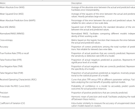
2.5 Performance metrics and model validation

Table 2Performance metrics for accuracy validation

Metric Description

Mean Absolute Error (MAE) Average of the absolute error between the actual and predicted values. Facilitates error interpretability.

Mean Squared Error (MSE) Average of the squares of the error between the actual and predicted values. Heavily penalizes large errors.

Mean Absolute Prediction Error (MAPE) Percentage of the error between the actual and predicted values. Not reliable for zero values or low-scale data.

Root MSE (RMSE) Squared root of MSE. Represents the standard deviation of the error between the actual and predicted values.

Normalized RMSE (NRMSE) Normalized RMSE. Facilitates comparing different models indepen-dently of their working scale.

Cross-entropy Metric based on the logistic function that measures the error between the actual and predicted values.

Accuracy Proportion of correct predictions among the total number of predic-tions. Not reliable for skewed class-wise data.

True Positive Rate (TPR) or recall Proportion of actual positives that are correctly predicted. Represents the sensitivity or detection rate (DR) of a model.

False Positive Rate (FPR) Proportion of actual negatives predicted as positives. Represents the significance level of a model.

True Negative Rate (TNR) Proportion of actual negatives that are correctly predicted. Represents the specificity of a model.

False Negative Rate (FNR) Proportion of actual positives predicted as negatives. Inversely propor-tional to the statistical power of a model.

Received Operating Characteristic (ROC) Curve that plots TPR versus FPR at different parameter settings. Facili-tates analyzing the cost-benefit of possibly optimal models.

Area Under the ROC Curve (AUC) Probability of confidence in a model to accurately predict positive outcomes for actual positive instances.

Precision Proportion of positive predictions that are correctly predicted.

F-measure Harmonic mean of precision and recall. Facilitates analyzing the trade-off between these metrics.

Coefficient of Variation (CV) Intra-cluster similarity to measure the accuracy of unsupervised classifi-cation models based on clusters.

Let us consider the accuracy validation of ML models for prediction. Usually, this accuracy validation undergoes an error analysis that computes the difference between the actual and predicted values. Recall, a prediction is an outcome of ML models for classification and regression problems. In classification, the common metrics for error analysis are based on the logistic function, such as binary and categorical cross-entropy—for binary and multi-class classification, respectively. In regression, the conventional error metrics are Mean Absolute Error (MAE) and Mean Squared Error (MSE). Both regression error metrics dis-regard the direction of under- and over-estimations in the predictions. MAE is simpler and easier to interpret than MSE, though MSE is more useful for heavily penalizing large errors.

The above error metrics are commonly used to com-pute the cost function of ML-based classification and regression models. Computing the cost function of the training and validation datasets (cf., Section 2.2) allow diagnosing performance problems due to high bias or

high variance. High bias refers to a simple ML model that poorly maps the relations between features and outcomes (under-fitting). High variance implies an ML model that fits the training data but does not generalize well to pre-dict new data (over-fitting). Depending on the diagnosed problem, the ML model can be improved by going back to one of the following design constituents (cf., Fig. 3): (i) data collection, for getting more training data (only for high variance), (ii) feature engineering, for increasing or reducing the set of features, and (iii) model learning, for building a simpler or more complex model, or for adjusting a regularization parameter.

(NRMSE). MAPE states the prediction error as a per-centage, while RMSE expresses the standard deviation of the error. Whereas, NRMSE allows comparing between models working on different scales, unlike the other error metrics described.

In classification, the conventional metric to report the performance of an ML model is the accuracy. The accu-racy metric is defined as the proportion of true

predic-tions T for each class Ci ∀i = 1...N among the total

number of predictions, as follows:

Accuracy=

N

i=1TCi Total Predictions

For example, let us consider a classification model that predicts whether an email should go to the spam, inbox, or promotion folder (i.e. multi-class classification). In this case, the accuracy is the sum of emails correctly predicted as spam, inbox, and promotion, divided by the total num-ber of predicted emails. However, the accuracy metric is not reliable when the data is skewed with respect to the classes. For example, if the actual number of spam and promotion emails is very small compared to inbox emails, a simple classification model that predictseveryemail as inbox will still achieve a high accuracy.

To tackle this limitation, it is recommended to use the metrics derived from a confusion matrix, as illustrated in Fig.4. Consider that each row in the confusion matrix rep-resents a predicted outcome and each column reprep-resents the actual instance. In this manner, True Positive (TP) is the intersection between correctly predicted outcomes for the actual positive instances. Similarly, True Negative (TN) is when the classification model correctly predicts an actual negative instance. Whereas, False Positive (FP) and False Negative (FN) describe incorrect predictions for negative and positive actual instances, respectively. Note, that TP and TN correspond to the true predictions for

Fig. 4Confusion matrix for binary classification

the positive and negative classes, respectively. Therefore, the accuracy metric can also be defined in terms of the confusion matrix:

Accuracy= TP+TN

TP+TN+FP+FN

The confusion matrix in Fig.4works for a binary clas-sification model. Therefore, it can be used in multi-class classification by building the confusion matrix for a spe-cific class. This is achieved by transforming the multi-class classification problem into multiple binary classification

subproblems, using the one-vs-rest strategy. For

exam-ple, in the email multi-class classification, the confusion matrix for the spam class sets the positive class as spam and the negative class as the rest of the email classes (i.e. inbox and promotion), obtaining a binary classification model for spam and not spam email.

Consequentially, the True Positive Rate (TPR) describ-ing the number of correct predictions is inferred from the confusion matrix as:

TPR(Recall)= TP

TP+FN

The converse, False Positive Rate (FPR) is the ratio of incorrect predictions and is defined as:

FPR= FP

FP+TN

Similarly, True Negative Rate (TNR) and False Negative Rate (FNR) are used to deduce the number of correct and incorrect negative predictions, respectively. The terms recall,sensitivity, anddetection rate (DR)are often used to refer to TPR. In contrast, a comparison of the TPR versus FPR is depicted in a Received Operating Characteristics

(ROC) graph. In a ROC graph, where TPR is on the y

-axis and FPR is on thex-axis, a good classification model will yield a ROC curve that has a highly positive gradi-ent. This implies high TP for a small change in FP. As the gradient gets closer to 1, the prediction of the ML model deteriorates, as the number of correct and incorrect pre-dictions is approximately the same. It should be noted that a classification model with a negative gradient in the ROC curve can be easily improved by flipping the predictions from the model [16] or swapping the labels of the actual instances.

Precision= TP

TP+FP

The trade-off between recall and precision values allows to tune the parameters of the classification models and achieve the desired results. For example, in the binary spam classifier, a higher recall would avoid missing too many spam emails (lower FN), but would incorrectly pre-dict more emails as spam (higher FP). Whereas, a higher precision would reduce the number of incorrect predic-tions of emails as spam (lower FP), but would miss more spam emails (higher FN). F-measure allows to analyze the trade-off between recall and precision by providing the harmonic average, ideally 1, of these metrics:

F–measure=2· Precision·Recall Precision+Recall

The Coefficient of Variation (CV) is another accuracy metric, particularly used for reporting the performance of unsupervised models that conduct classification using clusters (or states). CV is a standardized measure of dis-persion that represents the intra-cluster (or intra-state) similarity. A lower CV implies a small variability of each outcome in relation to the mean of the corresponding cluster. This represents a higher intra-cluster similarity and a higher classification accuracy.

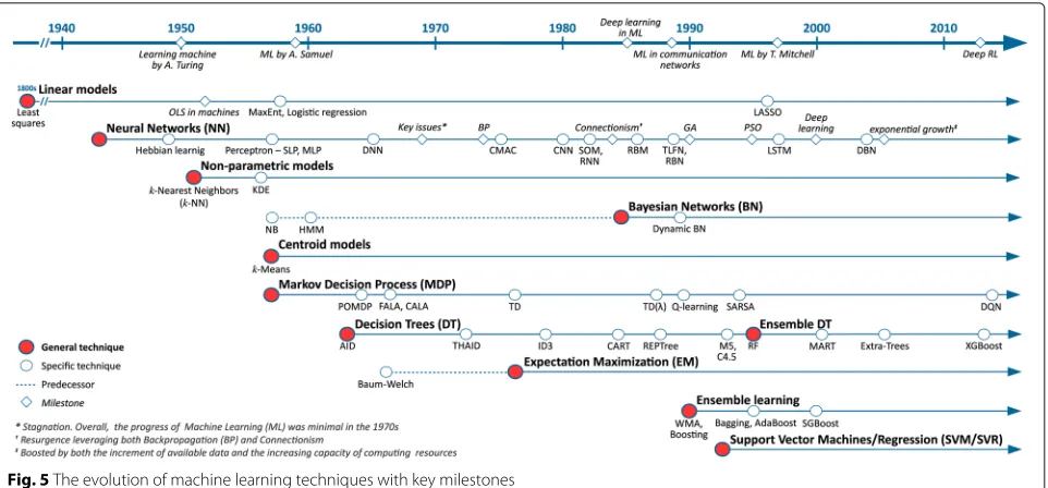
2.6 Evolution of machine learning techniques

Machine learning is a branch of artificial intelligence whose foundational concepts were acquired over the years from contributions in the areas of computer science, mathematics, philosophy, economics, neuroscience, psy-chology, control theory, and more [397]. Research efforts during the last 75 years have given rise to a plethora of ML techniques [15,169,397,435]. In this section, we pro-vide a brief history of ML focusing on the techniques that have been particularly applied in the area of computer networks (cf., Fig.5).

The beginning of ML dates back to 1943, when the first mathematical model of NNs for computers was pro-posed by McCulloch [302]. This model introduced a basic unit called artificial neuron that has been at the cen-ter of NN development to this day. However, this early model required to manually establish the correct weights of the connections between neurons. This limitation was addressed in 1949 by Hebbian learning [184], a simple rule-based algorithm for updating the connection weights of the early NN model. Like the neuron unit, Hebbian learning greatly influenced the progress of NN. These two concepts led to the construction of the first NN com-puter in 1950, called SNARC (Stochastic Neural Analog Reinforcement Computer) [397]. In the same year, Alan Turing proposed a test –where a computer tries to fool

a human into believing it is also human– to determine if a computer is capable of showing intelligent behavior. He described the challenges underlying his idea of a“learning machine”in [449]. These developments encouraged many researchers to work on similar approaches, resulting in two decades of enthusiastic and prolific research in the ML area.

In the 1950s, the simplest linear regression model called Ordinary Least Squares (OLS) –derived from the least squares method [266, 423] developed around the 1800s– was used to calculate linear regressions in electro-mechanical desk calculators [168]. To the best of our knowledge, this is the first evidence of using OLS in com-puting machines. Following this trend, two linear models for conducting classification were introduced: Maximum Entropy (MaxEnt) [215,216] and logistic regression [105]. A different research trend centered on pattern recognition exposed two non-parametric models (i.e. not restricted to a bounded set of parameters) capable of performing regression and classification:k-Nearest Neighbors (k-NN) [147, 420] and Kernel Density Estimation (KDE) [388],

also known as Parzen density [349]. The former uses

a distance metric to analyze the data, while the latter applies a kernel function (usually, Gaussian) to estimate the probability density function of the data.

The 1950s also witnessed the first applications of the Naïve Bayes (NB) classifier in the fields of pattern recog-nition [97] and information retrieval [297]. NB, whose foundations date back to the 18th and 19th centuries [43, 261], is a simple probabilistic classifier that applies Bayes’ theorem on features with strong independence assumptions. NB was later generalized using KDE, also known as NB with Kernel Estimation (NBKE), to estimate the conditional probabilities of the features. In the area of clustering, Steinhaus [422] was the first to propose a continuous version of the to be calledk-Means algorithm [290], to partition a heterogeneous solid with a given internal mass distribution into k subsets. The proposed centroid model employs a distance metric to partition the data into clusters where the distance to the centroid is minimized.

Fig. 5The evolution of machine learning techniques with key milestones

and one output layer, and Multi-Layer Perceptron (MLP), an NN with one or more hidden layers between the input and the output layers. The perceptron model is also known as Feedforward NN (FNN) since the nodes from each layer exhibit directed connections only to the nodes of the next layer. In the remainder of the paper, MLP-NNs and NNs in general, will be denoted by the tuple(input_nodes,hidden_layer_nodes+,output_nodes), for instance a (106, 60, 40, 1) MLP-NN has a 160-node input layer, two hidden layers of 60 and 40 nodes respec-tively, and a single node output layer.

By the end of the 1950s, the term“Machine Learning”

was coined and defined for the first time by Arthur Samuel (cf., Section 2), who also developed a checkers-playing game that is recognized as the earliest self-learning

pro-gram [401]. ML research continued to flourish in the

1960s, giving rise to a novel statistical class of the Markov

model, named Hidden Markov Model (HMM) [426]. An

HMM describes the conditional probabilities between hidden states and visible outputs in a partially observable, autonomous environment. The Baum-Welch algorithm [41] was proposed in the mi-1960s to learn those condi-tional probabilities. At the same time, MDP continued to instigate various research efforts. The partially observable Markov decision process (POMDP) approach to finding optimal or near-optimal control strategies for partially observable stochastic environments, given a complete model of the environment, was first proposed by Cassandra et al. [25] in 1965, while the algorithm to find the optimal solution was only devised 5 years later [416]. Another development in MDP was the learning automata –officially published in 1973 [448]–, a Reinforcement Learning (RL) technique that continuously updates the

probabilities of taking actions in an observed environ-ment, according to given rewards. Depending on the nature of the action set, the learning automata is classi-fied as Finite Action-set Learning Automata (FALA) or Continuous Action-set Learning Automata (CALA) [330]. In 1963, Morgan and Sonquis published Automatic Interaction Detection (AID) [323], the first regression tree algorithm that seeks sequential partitioning of an observa-tion set into a series of mutually exclusive subsets, whose means reduces the error in predicting the dependent vari-able. AID marked the beginning of the first generation of Decision Trees (DT). However, the application of DTs to classification problems was only initiated a decade later

by Morgan and Messenger’s Theta AID (THAID) [305]

algorithm.

In the meantime, the first algorithm for training MLP-NNs with many layers –also known as Deep NN (DNN) in today’s jargon– was published by Ivakhnenko and Lapa

in 1965 [210]. This algorithm marked the

commence-ment of the Deep Learning (DL) discipline, though the term only started to be used in the 1980s in the general context of ML, and in the year 2000 in the specific

con-text of NNs [9]. By the end of the 1960s, Minsky and

Papertkey’s Perceptronsbook [315] drew the limitations of perceptrons-based NN through mathematical analysis, marking a historical turn in AI and ML in particular, and significantly reducing the research interest for this area over the next several years [397].

Although ML research was progressing slower than

projected in the 1970s [397], the 1970s were marked

Cerebellar Model Articulation Controller (CMAC) NN

model [11], the Expectation Maximization (EM)

algo-rithm [115], the to-be-referred-to as Temporal Difference (TD) learning [478], and the Iterative Dichotomiser 3 (ID3) algorithm [373].

Werbos’s application of BP –originally a control theory algorithm from the 1960s [80,81,233]– to train NNs [472] resurrected the research in the area. BP is to date the most popular NN training algorithm, and comes in different variants such as Gradient Descent (GD), Conjugate Gra-dient (CG), One Step Secant (SS), Levenberg-Marquardt (LM), and Resilient backpropagation (Rp). Though, BP is widely used in training NNs, its efficiency depends on the choice of initial weights. In particular, BP has been shown to have slower speed of convergence and to fall into local optima. Over the years, global optimization methods have been proposed to replace BP, including Genetic Algo-rithms (GA), Simulated Annealing (SA), and Ant Colony (AC) algorithm [500]. In 1975, Albus proposed CMAC, a new type of NN as an alternative to MLP [11]. Although CMAC was primarily designed as a function modeler for robotic controllers, it has been extensively used in RL and classification problems for its faster learning compared to MLP.

In 1977, in the area of statistical learning, Dempster et al. proposed EM, a generalization of the previous iter-ative, unsupervised methods, such as the Baum-Welch algorithm, for learning the unknown parameters of

sta-tistical HMM models [115]. At the same time, Witten

developed an RL approach to solve MDPs, inspired by ani-mal behavior and learning theories [478], that was later referred to as Temporal Difference (TD) in Sutton’s work [433,434]. In this approach the learning process is driven by the changes, or differences, in predictions over succes-sive time steps, such that the prediction at any given time step is updated to bring it closer to the prediction of the same quantity at the next time step.

Towards the end of the 1970s, the second generation of DTs emerged as the Iterative Dichotomiser 3 (ID3) algo-rithm was released. The algoalgo-rithm, developed by Quinlan [373], relies on a novel concept for attribute selection based on entropy maximization. ID3 is a precursor to the popular and widely used C4.5 and C5.0 algorithms.

The 1980s witnessed a renewed interest in ML research, and in particular in NNs. In the early 1980s, three new classes of NNs emerged, namely Convolutional Neural Network (CNN) [157], Self-Organizing Map (SOM) [249],

and Hopfield network [195]. CNN is a feedforward NN

specifically designed to be applied to visual imagery anal-ysis and classification, and thus require minimal image preprocessing. Connectivity between neurons in CNN is inspired by the organization of the animal visual cortex –modeled by Hubel in the 1960s [200,201]–, where the visual field is divided between neurons, each responding

to stimuli only in its corresponding region. Similarly to CNN, SOM was also designed for a specific application domain; dimensionality reduction [249]. SOMs employ an unsupervised competitive learning approach, unlike tra-ditional NNs that apply error-correction learning (such as BP with gradient descent).

In 1982, the first form of Recurrent Neural Network (RNN) was introduced by Hopfield. Named after the inventor, Hopfield network is an RNN where the weights connecting the neurons are bidirectional. The modern definition of RNN, as a network where connections between neurons exhibit one or more than one cycle,

was introduced by Jordan in 1986 [226]. Cycles

pro-vide a structure for internal states or memory allow-ing RNNs to process arbitrary sequences of inputs. As such, RNNs are found particularly useful in Time Series Forecasting (TSF), handwriting recognition and speech recognition.

Several key concepts emerged from the 1980s’

con-nectionism movement, one of which is the concept of distributed representation[187]. Introduced by Hinton in 1986, this concept supports the idea that a system should be represented by many features and that each feature may have different values. Distributed representation estab-lishes a many-to-many relationship between neurons and (feature,value)pairs for improved efficiency, such that a (feature,value)input is represented by a pattern of activity across neurons as opposed to being locally represented by a single neuron. The second half of 1980s also witnessed the increase in popularity of the BP algorithm and its suc-cessful application in training DNNs [263,394], as well as the emergence of new classes of NNs, such as Restricted

Boltzmann Machines (RBM) [413], Time-Lagged

Feedfor-ward Network (TLFN) [260], and Radial Basis Function

Neural Network (RBFNN) [260].

Originally named Harmonium by Smolensky, RBM is a variant of Boltzmann machines [2] with the restric-tion that there are no connecrestric-tions within any of the network layers, whether it is visible or hidden. Therefor, neurons in RBMs form a bipartite graph. This restric-tion allows for more efficient and simpler learning com-pared to traditional Boltzmann machines. RBMs are found useful in a variety of application domains such as dimensionality reduction, feature learning, and classifi-cation, as they can be trained in both supervised and unsupervised ways. The popularity of RBMs and the extent of their applicability significantly increased after the mid-2000s as Hinton introduced in 2006 a faster learning method for Boltzmann machines called Con-trastive Divergence [186] making RBMs even more attrac-tive for deep learning [399]. Interestingly, although the use of the term “deep learning” in the ML community

dates back to 1986 [111], it did not apply to NNs at

Towards the end of 1980s, TLFN –an MLP that incor-porates the time dimension into the model for conducting

TSF [260]–, and RBFNN –an NN with a weighted set of

Radial Basis Function (RBF) kernels that can be trained in unsupervised and supervised ways [78]– joined the grow-ing list of NN classes. Indeed any of the above NNs can be employed in a DL architecture, either by implement-ing a larger number of hidden layers or stackimplement-ing multiple simple NNs.

In addition to NNs, several other ML techniques thrived during the 1980s. Among these techniques, Bayesian Net-work (BN) arose as a Directed Acyclic Graph (DAG) representation model for the statistical models in use

[352], such as NB and HMM –the latter considered as

the simplest dynamic BN [107,110]–. Two DT learning algorithms, similar to ID3 but developed independently, referred to as Classification And Regression Trees (CART) [76], were proposed to model classification and regres-sion problems. Another DT algorithm, under the name of Reduced Error Pruning Tree (REPTree), was also intro-duced for classification. REPTree aimed at building faster and simpler tree models using information gain for split-ting, along with reduced-error pruning [374].

Towards the end of 1980s, two TD approaches were proposed for reinforcement learning: TD(λ) [433] and Q-learning [471]. TD(λ) adds a discount factor (0≤λ ≤1) that determines to what extent estimates of previous state-values are eligible for updating based on current errors, in the policy evaluation process. For example, TD(0) only updates the estimate of the value of the state preced-ing the current state. Q-learnpreced-ing, however, replaces the traditional state-value function of TD by an action-value function (i.e. Q-value) that estimates the utility of taking a specific action in specific states. As of today, Q-learning is the most well-studied and widely-used model-free RL algorithm. By the end of the decade, the application domains of ML started expending to the operation and management of communication networks [57,217,289].

In the 1990s, significant advances were realized in ML research, focusing primarily on NNs and DTs. Bio-inspired optimization algorithms, such as Genetic Algo-rithms (GA) and Particle Swarm Optimization (PSO), received increasing attention and were used to train NNs for improved performance over the traditional BP-based learning [234,319]. Probably one of the most important achievements in NNs was the work on Long Short-Term Memory (LSTM), an RNN capable of learning long-term dependencies for solving DL tasks that involve long input sequences [192]. Today, LSTM is widely used in speech recognition as well as natural language processing. In DT research, Quinlan published the M5 algorithm in 1992 [375] to construct tree-based multivariate linear models analogous to piecewise linear functions. One well-known variant of the M5 algorithm is M5P, which aims at building

trees for regression models. A year later, Quinlan

pub-lished C4.5 [376], that builds on and extends ID3 to

address most of its practical shortcomings, including data overfitting and training with missing values. C4.5 is to date one of the most important and widely used algorithms in ML and data mining.

Several techniques other than NN and DT also pros-pered in the 1990s. Research on regression analysis propounded the Least Absolute Selection and Shrink-age Operator (LASSO), which performs variable selec-tion and regularizaselec-tion for higher predicselec-tion accuracy

[445]. Another well-known ML technique introduced in

the 1990s was Support Vector Machines (SVM). SVM enables plugging different kernel functions (e.g. linear, polynomial, RBF) to find the optimal solution in higher-dimensional feature spaces. SVM-based classifiers find a hyperplane to discriminate between categories. A single-class SVM is a binary single-classifier that deduces the hyper-plane to differentiate between the data belonging to the class against the rest of the data, that is, one-vs-rest. A multi-class approach in SVM can be formulated as a series of single class classifiers, where the data is assigned to the class that maximizes an output function. SVM has been widely used primarily for classification, although a regres-sion variant exists, known as Support Vector Regresregres-sion (SVR) [70].

In the area of RL, SARSA (State-Action-Reward-State-Action) was introduced as a more realistic, however less practical, Q-learning variation [395]. Unlike Q-learning, SARSA does not update the Q-value of an action based on the maximum action-value of the next state, but instead it uses the Q-value of the action chosen in the next state.

A new emerging concept called ensemble learning

demonstrated that the predictive performance of a single learning model can be be improved when combined with other models [397]. As a result, the poor performance of a single predictor or classifier can be compensated with ensemble learning at the price of (significantly) extra computation. Indeed the results from ensemble learning must be aggregated, and a variety of techniques have been proposed in this matter. The first instances of ensemble learning include Weighted Majority Algorithm (WMA) [279], boosting [403], bootstrap aggregating (or bagging) [75], and Random Forests (RF) [191]. RF focused explic-itly on tree models and marked the beginning of a new generation of ensemble DT. In addition, some variants of the original boosting algorithm were also developed, such

as Adaptive Boosting (AdaBoost) [153] and Stochastic

Gradient Boosting (SGBoost) [155].

finance, manufacturing, medicine, science) for processing huge amounts of data to build models with valuable use [169]. Furthermore, from a conceptual perspective, Tom Mitchell formally defined ML: “A computer program is said to learn from experienceEwith respect to some class of tasksTand performance measureP, if its performance at tasks inT, as measured byP, improves with experience E” [317].

The 21st century began with a new wave of increasing interest in SVM and ensemble learning, and in partic-ular ensemble DT. Research efforts in the field gener-ated some of the the most widely used implementations of ensemble DT as of today: Multiple Additive Regres-sion Trees (MART) [154], extra-trees [164], and eXtreme

Gradient Boosting (XGBoost) [93]. MART and XGBoost

are respectively a commercial and open source imple-mentation of Friedman’s Gradient Boosting Decision Tree (GBDT) algorithm; an ensemble DT algorithm based on gradient boosting [154, 155]. Extra-trees stands for extremely randomized trees, an ensemble DT algorithm

that builds random trees based on k randomly chosen

features. However instead to computing an optimal split-point for each one of thek features at each node as in RF, extra-trees selects a split-point randomly for reduced computational complexity.

At the same time, the popularity of DL increased signif-icantly after the term “deep learning” was first introduced in the context of NNs in 2000 [9]. However, the attrac-tiveness of DNN started decreasing shortly after due to the experienced difficulty of training DNNs using BP (e.g. vanishing gradient problem), in addition to the increas-ing competitiveness of other ML techniques (e.g. SVM)

[169]. Hinton’s work on Deep Belief Networks (DBN),

published in 2006 [188], gave a new breath and strength to research in DNNs. DBN introduced an efficient train-ing strategy for deep learntrain-ing models, which was further used successfully in different classes of DNNs [49, 381]. The development in ML –particularly, in DNNs– grew exponentially with advances in storage capacity and large-scale data processing (i.e. Big Data) [169]. This wave of popularity in deep learning has continued to this day, yielding major research advances over the years. One approach that is currently receiving tremendous atten-tion is Deep RL, which incorporates deep learning models into RL for solving complex problems. For example, Deep Networks (DQN) –a combination of DNN and Q-learning– was proposed for mastering video games [318]. Although the term Deep RL was coined recently, this concept was already discussed and applied 25 years ago [275,440]. It is important to mention that the evolution in ML research has enabled improved learning capabilities which were found useful in several application domains, ranging from games, image and speech recognition, network oper-ation and management, to self-driving cars [120].

3 Traffic prediction

Network traffic prediction plays a key role in network operations and management for today’s increasingly com-plex and diverse networks. It entails forecasting future traffic and traditionally has been addressed via time series forecasting (TSF). The objective in TSF is to construct a regression model capable of drawing accurate correlation between future traffic volume and previously observed traffic volumes.

Existing TSF models for traffic prediction can be broadly decomposed into statistical analysis models and supervised ML models. Statistical analysis models are typ-ically built upon the generalized autoregressive integrated moving average (ARIMA) model, while majority of learn-ing for traffic prediction is achieved via supervised NNs. Generally, the ARIMA model is a popular approach for TSF, where autoregressive (AR) and moving average (MA) models are applied in tandem to perform auto-regression on the differenced and “stationarized” data. However, with the rapid growth of networks and increasing complexity of network traffic, traditional TSF models are seemingly compromised, giving rise to more advanced ML models. More recently, efforts have been made to reduce overhead and, or improve accuracy in traffic prediction by employ-ing features from flows, other than traffic volume. In the following subsections, we discuss the various traffic pre-diction techniques that leverage ML and summarize them in Table3.

3.1 Traffic prediction as a pure TSF problem

To the best of our knowledge, Yu et al. [489] were the first to apply ML in traffic prediction using MLP-NN. Their primary motive was to improveaccuracyover traditional AR methods. This was supported by rigorous independent mathematical proofs published in the late eighties and the early nineties by Cybenko [106], Hornik [196], and Funa-hashi [158]. These proofs showed that SLP-NN approxi-mators, which employed sufficient number of neurons of continuous sigmoidal activation type (a constraint intro-duced by Cybenko and relaxed by Hornik), were universal approximators, capable of approximating any continuous function to any desired accuracy.

In the last decade, different types of NNs (SLP, MLP, RNN, etc.) and other supervised techniques have been employed for TSF of network traffic. Eswaradass et al.

[141] propose a MLP-NN-based bandwidth prediction

system for Grid environments and compare it to the

Network Weather Service (NWS) [480] bandwidth

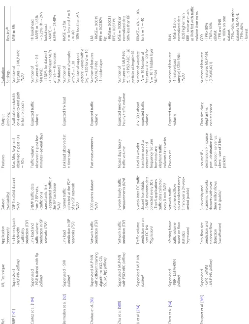
Table 3 Summary of TSF and non-TSF-based traffic prediction Ref. ML Technique A pplication D ataset Features O utput Evaluation (approach) (availability) (training) Settings Results ab NBP [ 141 ]

Supervised: ·MLP-NN

(offline)

End-to-end

path

bandwidth availability prediction

(TSF) NSF TeraGrid dataset (N/A) Max, M in, A vg load observed in past 10 s ∼ 30 s Available b andwidth on a e nd-to-end path in future epoch Number of features = 3 M LP-NN: · (N/A) MSE = 8% Cortez et al. [ 104 ]

Supervised: ·NNE

trained with Rp (offline) Link load and traffic volume prediction in ISP networks (TSF) SNMP traffic data from 2 ISP nets, · traffic o n a transatlantic link · aggregated traffic in the ISP backbone (N/A) Traffic volume observed in past few minutes ∼ several days Expected traffic volume Number of features = 6 ∼ 95 NNs NNE: · all SLPs for dataset1 · 1 h idden layer MLPs with 6 ∼ 8n e u ro n s for dataset2 1h lookahead: · MAPE = 1.43% ∼ 5.23% 1h ∼ 24h

lookahead: ·MAPE

= 6.34% ∼ 23.48% Bermolen et al. [ 52 ] Supervised: · SVR (offline) Link load prediction in ISP networks (TSF) Internet traffic collected at the P OP of an ISP n etwork (N/A) Link load observed at τ time scale Expected link load Number of features = d samples with d = 1..30 Number of support vectors: · varies with d (e.g. ∼ 320 for d = 10) RMSE < 2 for τ = 1 ms and d = 5 ·≈ AR · 10% less than MA Chabaa et al. [ 86 ] Supervised: M LP-NN with d ifferent training algorithms (GD, CG, SS, LM, R p) (offline) Network traffic prediction (TSF) 1000 points dataset (N/A) Past measurements Expected traffic volume Number of features (N/A) MLP-NN: · 1 h idden layer

LM: ·RMSE

=

0.0019

RPE

=

0.0230%

Rp: ·RMSE

= 0.0031 RPE = 0.0371% Zhu e t al. [ 500 ] Supervised: M LP-NN with P SO-ABC (offline) Network traffic prediction (TSF) 2-week hourly traffic measurements (N/A) N p ast days h ourly traffic volume Expected next-day hourly traffic volume Number of features = 5 M LP-NN (5, 11, 1) PSO-ABC: · 30 particles o fl ength=66 MSE = 0.006 on normalized data 50% less than BP Li et al. [ 274 ] Supervised: M LP-NN (offline) Traffic volume prediction on an inter-DC link (Regression) 6-week inter-DC traffic dataset from B aidu · SNMP counters data collected every 3 0 s · Top-5 applications traffic data collected every 5 min (N/A) Level-N w avelet transform u sed to extract time and frequency features from total and elephant traffic volumes time series k × 30-s ahead expected traffic volume Number of wavelets: · N = 10 Number of features = k × 120 for N = 10 1 h idden layer MLP-NN RRMSE = 4% ∼ 10% for k = 1 ∼ 40 Chen et al. [ 94 ]

Supervised: ·KBR

· LSTM-RNN (offline) Inferring future traffic volume based o n flow statistics (regression) Network traffic volume and flow count collected every 5 m in over a 24-week period (public) Flow count Expected traffic volume Number of features: · 1 feature (past sample) LSTM-RNN: · (N/A)

RNN ·MSE

> 0.3 o n normalized data · 0.05 higher than KBR · twice as much as RNN fed with traffic volume time series P o u p ar te ta l. [ 365 ]

Supervised: ·GPR

· oBMM · MLP-NN (offline) Early flow-size prediction and elephant flow detection (classification) 3 university and academic n etworks datasets with o ver three m illion flows each (public) · source IP · destination IP · source port · destination p ort · protocol · server vs. client · size of 3 first packets Flow size class; elephant vs. non-elephant Number of features: · 7 features M LP-NN: · (106,60,40,1)

GPR: ·TPR

> 80% · TNR > 80%

oBMM: ·TPR

and TNR ≈ 100% on one

dataset ·TPR

< 50% o n o ther datasets MLP-NN: · TPR > 80% ·

lowest _TNR<

40 gigabit/s NSF TeraGrid network datasets show that the NN outperforms the NWS bandwidth forecasting models with an error rate of up to 8 and 121.9% for MLP-NN and NWS, respectively. Indeed the proposed NN-based fore-casting system shows better learning ability than NWS’s. However, no details are provided for the characteristics of the MLP employed in the study, nor the time complexity of the system compared to NWS.

Cortez et al. [104] choose to use a NN ensemble (NNE) of five MLP-NN with one hidden layer each. Resilient backpropagation (Rp) training is used on SNMP traffic data collected from two different ISP networks. The first data represents the traffic on a transatlantic link, while the second represents the aggregated traffic in the ISP back-bone. Linear interpolation is used to complete missing

SNMP data. The NNE is tested forreal-timeforecasting

(online forecasting on a few-minute sample),short-term

(one-hour to several-hours sample), and mid-term

fore-casting (one-day to several-days sample). The NNE is compared against AR models of traditional Holt-Winters, double Holt-Winters seasonal variant to identify repe-titions in patterns at fixed time periods, and ARIMA. The comparison amongst the TSF methods show that in general the NNE produces the lowest MAPE for both datasets. It also shows that in terms of time and compu-tational complexity, NNE outperforms the other methods with an order of magnitude, and is well suited for real-time forecasting.

The applicability of NNs in traffic prediction instigated various other efforts [86, 500] to compare and contrast various training algorithms for network traffic prediction. Chabaa et al. [86] evaluate the performance of various BP training algorithms to adjust the weights in the MLP-NN, when applied to Internet traffic time series. They show superior performance, with respect to RMSE and RPE, of the Levenberg-Marquardt (LM) and the Resilient back-propagation (Rp) algorithms over other BP algorithms.

In contrast to the local optimization in BP, Zhu et al. [500] propose a hybrid training algorithm that is based on global optimization, the PSO-ABC technique [98]. It is an artificial bee colony (ABC) algorithm employing par-ticle swarm optimization (PSO), an evolutionary search algorithm. The training algorithm is implemented with a

(5, 11, 1)MLP-NN. Experiments on a 2 weeks hourly traf-fic measurement dataset show that PSO-ABC has higher prediction accuracy than BP, with an MSE of 0.006 and 0.011, respectively, on normalized data and has stable pre-diction performance. Furthermore, the hybrid PSO-ABC has a faster training time than ABC or PSO.

On the other hand, SVM has a low computational over-head and is more robust to parameter variations (e.g. time scale, number of samples) in general. However, they are usually applied to classification rather than TSF. SVM and its regression variant, SVR, are scrutinized for their

applicability to traffic prediction in [52]. Bermolen et al. [52] consider the prospect of applying SVR for link load forecasting. The SVR model is tested on heterogeneous Internet traffic collected at the POP of an ISP network. At 1sec timescale, the SVR model shows a slight improve-ment over an AR model in terms of RMSE. A more sig-nificant 10% improvement is achieved over a MA model. Most importantly, SVR is able to achieve 9000 forecast per sec with 10 input samples, and shows the potential for real-time operation.

3.2 Traffic prediction as a non-TSF problem

In contrast to TSF methods, network traffic can be predicted leveraging other methods and features. For instance, Li et al. [274] propose a frequency domain based method for network traffic flows, instead of just traffic volume. The focus is on predicting incoming and out-going traffic volume on an inter-data center link domi-nated by elephant flows. Their models incorporate FNN, trained with BP using simple gradient descent and wavelet transform to capture both the time and frequency fea-tures of the traffic time series. Elephant flows are added as separate feature dimensions in the prediction. How-ever, collecting all elephant flows at high frequencies is more expensive than byte count for traffic volume. There-fore, elephant flow information is collected at lower fre-quencies and interpolated to fill in the missing values, overcoming the overhead for elephant flow collection.

The dataset contains the total incoming and outgoing traffic collected in 30 s intervals using SNMP counters on the data center (DC) edge routers and inter-DC link at Baidu over a six-week period. The top 5 applications account for 80% of the total incoming and outgoing traffic data, which is collected every 5 min and interpolated to estimate missing values at the 30 s scale. The time series is decomposed using level 10 wavelet transform, leading to 120 features per timestamp.