Open Access
R E S E A R C H
© 2010 Rousson et al; licensee BioMed Central Ltd. This is an Open Access article distributed under the terms of the Creative Commons Attribution License (http://creativecommons.org/licenses/by/2.0), which permits unrestricted use, distribution, and reproduction in any medium, provided the original work is properly cited.
Research
A set of indicators for decomposing the secular
increase of life expectancy
Valentin Rousson* and Fred Paccaud
Abstract
Background: The ongoing increase in life expectancy in developed countries is associated with changes in the shape of the survival curve. These changes can be characterized by two main, distinct components: (i) the decline in premature mortality, i.e., the concentration of deaths around some high value of the mean age at death, also termed rectangularization of the survival curve; and (ii) the increase of this mean age at death, i.e., longevity, which directly reflects the reduction of mortality at advanced ages. Several recent observations suggest that both mechanisms are simultaneously taking place.
Methods: We propose a set of indicators aiming to quantify, disentangle, and compare the respective contribution of rectangularization and longevity increase to the secular increase of life expectancy. These indicators, based on a nonparametric approach, are easy to implement.
Results: We illustrate the method with the evolution of the Swiss mortality data between 1876 and 2006. Using our approach, we are able to say that the increase in longevity and rectangularization explain each about 50% of the secular increase of life expectancy.
Conclusion: Our method may provide a useful tool to assess whether the contribution of rectangularization to the secular increase of life expectancy will remain around 50% or whether it will be increasing in the next few years, and thus whether concentration of mortality will eventually take place against some ultimate biological limit.
Background
Life expectancy almost doubled in developed countries during the 20th century. This increase was initially related to the reduction in infant mortality. After the 1950 s, the increase was related to the decline in mortality in old age [1]. In both phases, the evolution is usually related to the combination of a massive improvement in the social and physical environment and to an improve-ment in health care. Whether the former improveimprove-ment had more effect on the decline of mortality than the latter (as suggested by McKeown's theory) is still a matter of debate [2]. No strong, comprehensive theory is yet avail-able to fully understand the past trends, and hence, the current and future evolution of human longevity. How-ever, several paradigms have been proposed to capture the underlying mechanisms at stake. One of them was provided by Fries in 1980 [3], relating the secular increase
of life expectancy to the postponement of age of death. This corresponds to the strong decline (or even the fad-ing) of premature mortality and morbidity, and to the concentration (or compression) of deaths around some fixed, optimal mean age at death value, estimated at 85 years. This evolution was coined as "rectangularization," suggesting that the final stage of the survival curve will be a perfect rectangle.
This paradigm developed by Fries was mainly based on visual inspection. Several authors developed quantitative indicators to capture the shape of the survival curves [4-8]. Most confirmed a concentration of age at death around high mean values with a decreasing variability. However, some papers showed a slowdown of rectangu-larization during the last decades, sometimes with a decline resuming after a plateau [9], while others found an increase in the variability of age at death over 60 years [10,11]. In the same line, others showed a continuous increase of the maximal age at death in the last century [1,12], with no signs of a finite life-span limit [13]. In the latter paper, Wilmoth explicitly suggested that rectangu-* Correspondence: [email protected]
1 Institute for Social and Preventive Medicine (IUMSP), University Hospital and Faculty of Medicine, Lausanne, Switzerland
larization of the survival curve and increase of longevity are in fact occurring simultaneously, i.e., that the distri-bution of age at death could become more and more compressed while also shifting further and further to the right. In order to evaluate and monitor this hypothesis, we propose in this paper a set of quantitative, nonpara-metric indicators, namely a rectangularity index and a longevity index, to quantify and disentangle the respec-tive contributions of rectangularization and longevity increase to the secular increase of life expectancy.
Methods
Wilmoth and Horiuchi [5] reviewed 10 measures charac-terizing either the rectangularity of a survival curve or the variability of age at death. One of these was coined "moving rectangle" and constructed as follows. Let S*(t)
be the survival curve from a cohort of interest, and let be a very high quantile of the distribution of age at death,
such that (Wilmoth and Horiuchi
consid-ered Q = .999). Consider a rectangle with lower-left and
upper-right corner coordinates (0,1 - Q) and ( , 1), thus
of dimension Q. A straightforward measure of rectan-gularity is given by the proportion of this rectangle lying below the survival curve, defined as:
Our approach is based on this indicator, and is devel-oped in three steps as follows.
The first step is to remove the impact of early mortality (infant, children, and young adults) to focus the analysis on the mortality of the most elderly. The rectangle is thus not drawn from birth, but from some pre-specified age, t0
(typically t0 = 50 years). The original survival curve S*(t)
is thus replaced by a survival curve S(t) conditional on age ≥ t0, defined such that S(t0 ) = 1, and a high quantile tQ of
the distribution of age at death conditional on age ≥ t0 is
then considered, identified such that S(tQ) = 1 - Q. In
order to get a more stable index, we do not use the maxi-mal age at death (i.e., Q = 1), nor an extremely high quan-tile of the distribution (e.g., Q = .99). A good compromise is Q =.9. The lower-left and upper-right corner coordi-nates of the modified "moving rectangle" are now given by (t0, 1 - Q) and (tQ, 1), with a dimension (tQ - t0)·Q. The
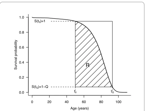
proportion of the rectangle lying below the conditional survival curve (see Figure 1) defines the "rectangularity index" R such as:
The higher R, the more rectangular the survival curve. In particular, R = 1 if the survival curve is perfectly rect-angular between t0 and tQ.
The second step is to define a "longevity index" as the quantile defined above, tQ. The higher tQ, the more
shifted to the right the survival curve.
The third step is to recognize that life expectancy con-ditional on age ≥t0 and on age ≤ tQ, noted CLEt0,Q, is a
simple function of the rectangularity index R and the lon-gevity index tQ. Let F(t) = 1-S(t) and f(t) = F'(t) be the
cumulative and density functions, respectively, of the conditional distribution of age at death. Integrating by parts, one obtains:
On the other hand, using the above definition of R, one has:
t*Q
S t*( Q*)= −1 Q
tQ*
tQ*
0 1 0
tQS t dt t tQ
Q Q
tQ Q
S t dt
tQ
*
*( ) * ( ) *
*( ) * *
∫ − ⋅ −
⋅ ≈ ∫
R
QS t dt tQ t Q
tQ t Q
t t
= ∫ − − ⋅ −
− ⋅
0 0 1
0
( ) ( ) ( )
( )
CLE
Qtf t dt
Q f t dt
tQQ QF t dt
Q
tQQ Q
t t
t t
t t
t t
t Q0 0
0
0
0
’
( )
( )
( ) = ∫
∫
= −∫
= +∫ SS t dt tQ t
Q
( ) −( − 0)
Figure 1 Example of survival curve with rectangularity index R
and longevity index tQ. These indexes are calculated from the
condi-tional survival curve S(t) for those people reaching the age of t0, such that S(t0 ) = 1 and S(tQ) = 1 - Q. On that example, t0 = 50, Q = 0.9, R = 0.66
and tQ = 92.
ending up with
In particular, for t0 = 0, CLE0,Q = R·tQ is simply the
prod-uct of both indexes.
From there, it is possible to decompose the differences between the CLEs of two survival curves as follows. Con-sider two curves with rectangularity indexes R(A) and R(B) and longevity indexes tQ(A) and tQ(B). The
corre-sponding CLEs are:
and
The difference between the two CLEs can be expressed as:
Thus, any difference between two CLEs is a sum of two terms. The first term is the difference of CLE, which would be obtained if the longevity index would remain constant, set at the average of tQ(A) and tQ(B). The second
term is the difference of CLE, which would be obtained if the rectangularity index would remain constant, set at the average of R(A) and R(B). In other words, the first term is interpreted as the part of the CLE difference attributable to a change of rectangularity, and the second term as the part attributable to a change of longevity.
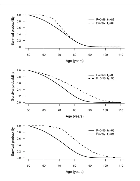
Hypothetical survival curves and patterns of change of CLE are shown in Figure 2, setting t0 = 50 years and Q = .9
in each panel. The solid line is a reference survival curve, established with R = .56 and tQ = 83 years, thus with a
corresponding CLE50,0.9 = 50 + .56(83 - 50) = 68.5 years.
The dashed lines correspond to three different patterns of increase in CLE compared to the reference curve. In the top panel, rectangularity index R increased from .56 to .67, while tQ is stable at 83 years. In the middle panel,
lon-gevity index tQ increased from 83 to 95 years, while R is
stable at .56. On the bottom panel, there is an increase of
both the rectangularity index R (from .56 to .67) and the longevity index tQ (from 83 to 95 years).
Thus, in the top panel, the increase of CLE from 68.5 years to 50 + .67(83 - 50) = 72.1 years is due to an increase of rectangularity only. In the middle panel, the increase of CLE from 68.5 years to 50 + .56 (95 - 50) = 75.2 years is due to an increase of longevity only. Finally, in the bottom panel, the increase of CLE from 68.5 years to 50 + .67 (95 - 50) = 80.2 years is due to both an increase of rectangu-larity and an increase of longevity. There, the difference of 11.7 years can be decomposed as:
In other words, 4.3 years (37% of the overall gain in CLE) are attributable to a difference in rectangularity, while the remaining 7.4 years (63%) are attributable to a difference in longevity. In what follows, we shall refer to "life expectancy difference attributable to rectangulariza-tion" (LEAR), the part (in %) of difference in CLE due to a change in rectangularity (in this example, LEAR = 37% ).
Results
The above approach has been applied to Swiss period life tables established by year of death for cohorts of men and women born in Switzerland between 1876 and 2006 [14]. The indicators above are implemented using t0 = 50 years
and Q = .9.
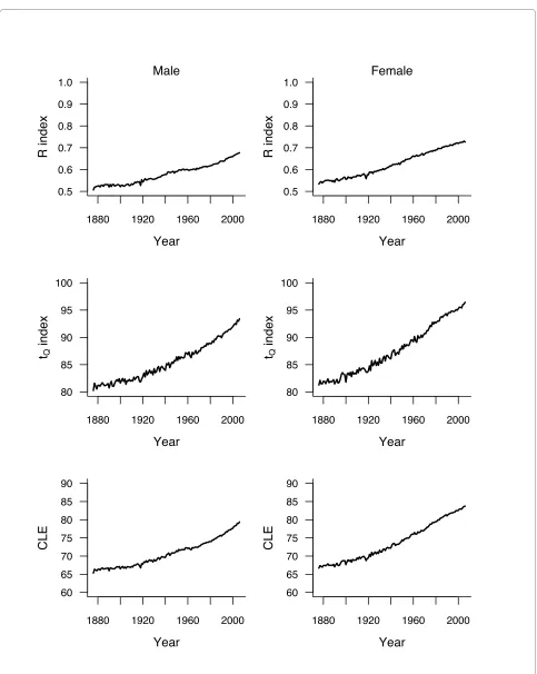
Figure 3 shows the survival curves for men and women for a sample of years. Rectangularity is visibly increasing over the century. This is reflected by an increasing R between 1876 and 2006, shifting from .51 to .68 for men and from .53 to .73 for women (upper panels of Figure 4). Figure 3 also shows a visible right shift of the curves, tQ
increasing during this period from 80 to 93 years for men and from 81 to 96 years for women (middle panels of Fig-ure 4). Overall, CLE50,0.9 increases by 14.1 years (from
65.3 to 79.4) for men and by 17.0 years (from 66.7 to 83.7) for women (bottom panels of Figure 4) between 1876 and 2006. Breaking up these differences shows that LEAR is similar in both sexes, slightly below 50% (namely, 45% for men and 44% for women). Thus, the increases in rectan-gularity and longevity contributed about equally to the increase in life expectancy.
The above analysis of mortality is using only the first and last year of the observation period. In order to explore the variation of LEAR over the years, we com-pared the CLE50,0.9 of two curves 20 years apart, i.e.,
com-paring 1896 to 1876, 1897 to 1877, etc., up to 2006 compared to 1986. Any other interval can be chosen, but a 20-year period is convenient because it corresponded approximately to one generation at the end of the 19th
S t dt tQ t R Q tQ t
t
tQ
( ) −( − )=( − ) ( − )
∫
0 1 00
CLEt Q tQ R tQ t t R tQ t
0, = +( −1)( − 0)= 0+ ( − 0)
CLEt Q A t R A tQ A t
0, ( )= 0+ ( )( ( )− 0)
CLEt Q0, ( )B =t0+R B t( )( Q( )B −t0)
CLE B CLE A
R B t B t R A t A t
R B
t Q t Q
Q Q
0 0
0 0
, ( ) , ( )
( )( ( ) ) ( )( ( ) )
( ( )
−
= − − −
= −RR A tQ A tQ B t
tQ B tQ A R A R B
( )) ( ) ( )
( ( ) ( )) ( ) ( )
⋅ + −
+ − ⋅⎛ +
⎝⎜
⎞ ⎠ ⎛
⎝
⎜ ⎞
⎠ ⎟ 2
2
0
⎟⎟
11 7 0 67 0 56 89 50 95 83 0 615 4 3 7 4
. ( . . )( ) ( ) .
. .
= − − + −
Figure 2 Examples of conditional survival curves, where an increase of conditional life expectancy (for those persons reaching t0 and dying
before tQ, with t0= 50 and Q = 0.9) is due to rectangularization only (top panel), due to longevity increase only (middle panel), or due to
both (bottom panel).
50 60 70 80 90 100 110
0.0 0.2 0.4 0.6 0.8 1.0
Age (years)
Survival probability
R=0.56 tQ=83
R=0.67 tQ=83
50 60 70 80 90 100 110
0.0 0.2 0.4 0.6 0.8 1.0
Age (years)
Survival probability
R=0.56 tQ=83 R=0.56 tQ=95
50 60 70 80 90 100 110
0.0 0.2 0.4 0.6 0.8 1.0
Age (years)
Survival probability
R=0.56 tQ=83
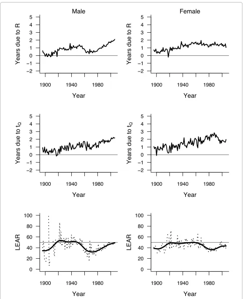
century. Eliciting shorter periods may lead to insignifi-cant gains that are difficult to interpret. The secular evo-lution of LEAR from 1896 to 2006 (the ends of the first and of the last 20-year period considered, respectively) is shown in the bottom panels of Figure 5. Note that LEAR was not calculated for those few years with a decrease of either the rectangularity index or the longevity index. Smoothing splines [15] have been added to improve the readability of the graphs.
Overall, there were few changes over the years, with LEAR fluctuating around means slightly under 50% in both genders. Fluctuations were slightly more marked for men than for women, and more marked before 1920 (likely because of the stronger annual variation of mortal-ity due to epidemics of communicable diseases). Overall, LEAR increased between 1876 and 1920, followed by a plateau and then by a decline since the 1940 s for men and since the 1960 s for women. LEAR was minimal (32%) for men in the 1970 s, and then increased slightly to below 50% at the turn of the century. For women, LEAR was minimal in the 1980 s at 36.5%, then increasing to 43% in 2006.
The same Figure 5 shows the secular trends in the num-ber of years gained in 20 years attributable to rectangular-ization (top panels) and to longevity increase (middle panels). It is important to note that the rhythm of increase accelerated over the period, although there is a decline and a plateau for the figures for women.
Obviously, the same indicators can be used to compare the survival curves from two populations at a given moment. For example, applying these indicators to com-pare men and women, one finds that the difference in CLE was 4.3 years in 2006, with about half (2.2 years, LEAR at 51%) attributable to a difference in rectangular-ity.
Discussion
This paper introduces the use of indicators characterizing the shape of a survival curve and measuring the impact of this shape on life expectancy. The first two indicators measure the rectangularity (R) and the longevity (tQ ) of
the survival curve at a given moment. The third indicator (LEAR) individualizes the impact of rectangularity and longevity on the differences in conditional life expectancy when comparing different moments or different popula-tions. Unlike many others, our indicators are nonpara-metric and do not rely on any model, such as Gompertz [16], logistic [17], or Gompertz mortality change models [18].
The index of rectangularity is based on the "moving rectangle," an idea explored by Wilmoth and Horiuchi [5]. It depends on two parameters, t0 and Q, which will in
turn affect the longevity index tQ . The method can use
any value of t0 and Q, although the values of the
indica-tors are sensitive to this choice. When choosing t0 = 40
instead of t0 = 50, for example, for the Swiss mortality
data from the previous section, the LEAR index compar-ing the years 1876 and 2006 is 48% for men and 46% for women instead of 45% and 44%. A similar comparison choosing t0 = 10 results in a LEAR index as high as 56%
for men and 55% for women. The choice of the parameter values should relate to the question under study. If, for example, the interest lies in longevity and old age mortal-ity, one should select a value for t0 high enough to remove
premature mortality (largely due to accidents). In devel-oped countries, a choice of t0 = 50 might be motivated by
the fact that it is usually at that age that degenerative dis-eases (such as cardiovascular disdis-eases or cancer) start to have some real impact. On the other hand, choosing Q = .9, i.e., removing the most elderly from the analysis, stabi-lizes the value of the longevity index (the index will not depend on a few persons, neither from the sample size if it is calculated using a sample of data instead of a life table). The resulting conditional life expectancy CLE50,0.9
is thus the mean age at death of those persons alive at 50 Figure 3 Survival curves estimated from life tables by year of
death (period) for cohorts of men (top panel) and women (bot-tom panel) born in Switzerland in 1876, 1900, 1925, 1950, 1975,
and 2006.
0 20 40 60 80 100
0.0 0.2 0.4 0.6 0.8 1.0 Age (years) Survival probability 2006 1975 1950 1925 1900 1876 Male 2006 1975 1950 1925 1900 1876 Male 2006 1975 1950 1925 1900 1876 Male 2006 1975 1950 1925 1900 1876 Male 2006 1975 1950 1925 1900 1876 Male 2006 1975 1950 1925 1900 1876 Male
0 20 40 60 80 100
Figure 4 Evolution of rectangularity index R (top panels) and longevity index tQ (middle panels), using t0 = 50 and Q = 0.9, estimated from
life tables by year of death (period) for cohorts of men (left panels) and women (right panels) born in Switzerland between 1876 and 2006. Bottom panels show the evolution of conditional life expectancy (for those persons reaching t0 and dying before tQ ) during that period.
1880 1920 1960 2000
0.5 0.6 0.7 0.8 0.9 1.0
Year
R index
Male
1880 1920 1960 2000
80 85 90 95 100
Year
t
Qindex
1880 1920 1960 2000
60 65 70 75 80 85 90
Year
CLE
1880 1920 1960 2000
0.5 0.6 0.7 0.8 0.9 1.0
Year
R index
Female
1880 1920 1960 2000
80 85 90 95 100
Year
t
Qindex
1880 1920 1960 2000
60 65 70 75 80 85 90
Year
Figure 5 Number of years gained (in conditional life expectancy compared to 20 years before) due to rectangularization (top panels) and
to longevity increase (middle panels), based on indexes R and tQwith t0 = 50 and Q = 0.9, estimated from life tables by year of death (period)
for cohorts of men (left panels) and women (right panels) born in Switzerland between 1876 and 2006. The dotted lines in the bottom panels
show the percentage of this gain attributable to rectangularization (LEAR). Smoothing splines have been added to show the trends (solid lines).
and dying before the 90th percentile of age at death for
this population. However, we do not exclude the possibil-ity that other authors might wish to apply the method using other values of t0 and Q, depending on their inter-est. Obviously, one should keep the same values for these parameters when comparing mortality in two different countries, or when evaluating the trend of the LEAR index along the years. Note that the corresponding parameters for the life expectancy at birth would be t0 = 0
and Q = 1.
Other nonparametric indicators have been proposed in the literature to measure the various dimensions of lifespan and high longevity. In their review, Wilmoth and Horiuchi [5] analyzed 10 indicators to measure either the rectangularity of the survival curve or the variability of the distribution of age at death (coined as "moving rect-angle", "fastest decline", "sharpest corner", or Keyfitz's H index), which were all highly correlated, such that these measures capture aspects of the shape of a survival curve that are strongly related. The authors concluded that one can choose one of them on the basis of convenience, and they favored the use of the interquartile range of age at death. Kannisto [6] further developed the idea, suggesting to consider the shortest age interval in which 50% of deaths take place as the best indicator of variability of age at death. Recognizing the need of having two indicators instead of one, Kannisto [7] finally proposed the modal age at death as a measure of longevity (which is in fact an alternative to our tQ ), in combination with the standard
deviation of the ages at death occurring above it as a mea-sure of variability (an alternative to R). Canudas-Romo [19] also considered the modal age at death, although in combination with the standard deviation around (not above) the mode.
The indicators proposed by Kannisto [7] have been recently applied by Cheung et al [20] to analyze the evolu-tion of life expectancy in Switzerland. With a decreasing standard deviation above modal age over the years, Che-ung et al concluded to a significant compression of adult mortality, at least from 1920. However, because modal age at death was still increasing without respite, their analysis did not find any evidence that we are approach-ing longevity limits in terms of maximum life span. As seen in the Results section, we could find similar conclu-sions using our indicators.
One possible advantage of considering our indicators R and tQ instead of those of Kannisto is that they can be
eas-ily (almost visually) calculated given any survival curve. In contrast, modal age at death is known to be difficult to estimate, and its appropriate determination is crucial [7,20]. The most substantial single advantage of using our indicators, however, is that they can be naturally com-bined with each other, allowing the proposed
decomposi-tion of a change of life expectancy and hence to separate and to compare the effects of rectangularization and lon-gevity increase to the secular increase of (conditional) life expectancy. This may be useful in the context of the debate initiated by Fries [3] as discussed in the Introduc-tion.
Conclusion
Analyzing the Swiss mortality data, our indicators sug-gest that the secular increase of life expectancy since the 1870 s is explained by the increase in both longevity and rectangularity, each responsible for about 50% of the increase. This corroborates Wilmoth's observation that both a rectangularization and an increase of longevity are simultaneously taking place [13]. It will be interesting to see whether the contribution of rectangularization to the secular increase of life expectancy will remain at around 50% or whether it will be increasing in the next few years. Also, a comparison among various industrialized and less industrialized countries with respect to this decomposi-tion, as well as an analysis of the factors associated with the impact of rectangularization, or with the one of lon-gevity increase on the decline of mortality, will be the subject of future research and should be of interest to many demographers.
Competing interests
The authors declare that they have no competing interests. Authors' contributions
The approach proposed in this paper is the result of numerous discussions between FP, who submitted the problem, and VR, who developed an initial version of the method. Both authors participated in the writing and editing of the manuscript. Both authors read and approved the final manuscript. Acknowledgements
We are grateful to Prof. Jean-Marie Robine for helpful discussions on an early phase of the manuscript.
Author Details
Institute for Social and Preventive Medicine (IUMSP), University Hospital and Faculty of Medicine, Lausanne, Switzerland
References
1. Robine JM, Paccaud F: Nonagenarians and centenarians in Switzerland, 1860-2001: a demographic analysis. Journal of Epidemiology and Community Health 2005, 59:31-37.
2. Colgrove J: The McKeown thesis: A historical controversy and its enduring influence. American Journal of Public Health 2002, 92:725-729. 3. Fries JF: Aging, natural death and the compression of morbidity. New
England Journal of Medicine 1980, 303:130-135.
4. Eakin T, Witten M: How square is the survival curve of a given species?
Experimental Gerontology 1995, 30:33-64.
5. Wilmoth JR, Horiuchi S: Rectangularization revisited: variability of age at death within human populations. Demography 1999, 36:475-495. 6. Kannisto V: Measuring the compression of mortality. Demographic
Research 2000, 3:Article 6.
7. Kannisto V: Mode and dispersion of the length of life. Population: An English Selection 2001, 13:159-171.
Received: 4 February 2010 Accepted: 9 June 2010 Published: 9 June 2010
This article is available from: http://www.pophealthmetrics.com/content/8/1/18 © 2010 Rousson et al; licensee BioMed Central Ltd.
8. Cheung SKL, Robine JM, Tu E, Caselli G: Three dimensions of the survival curve: horiontalization, verticalization, and longevity extension.
Demography 2005, 42:243-258.
9. Schneider EL, Brody JA: Aging, natural death and the compression of morbidity: another view. New England Journal of Medicine 1983, 309:854-856.
10. Myers GC, Manton KG: Compression of mortality: myth or reality? The Gerontologist 1984, 24:346-353.
11. Rothenberg R, Lentzner HR, Parker RA: Population aging patterns: the expansion of mortality. Journal of Gerontology 1991, 46:S66-70. 12. Wilmoth JR, Lundström H: Extreme longevity in five countries. European
Journal of Population 1996, 12:63-93.
13. Wilmoth JR: In search of limits: what do demographic trend suggests about the future of human longevity? In Between Zeus and the Salmon: The Biodemography of Longevity Edited by: Wachter KW and Fich CE. National Academy Press; 1997:38-64.
14. The Human Mortality Database Human Mortality Database [http:// www.mortality.org]. University of California, Berkeley (USA), and Max Planck Institute for Demographic Research (Germany) (data downloaded on October 8, 2008)
15. Chambers JM, Hastie TJ: Statistical Models in S Wadsworth & Brooks/Cole; 1992.
16. Strehler BL and Mildvan AS: General theory of mortality and aging.
Science 1960, 132:14-21.
17. Thatcher AR: The long-term pattern of adult mortality and the highest attained age. Journal of the Royal Statistical Society A 1999, 162:5-43. 18. Vaupel JW, Canudas-Romo V: Decomposing change in life expectancy:
A bouquet of formulas in honor of Nathan Keyfitz's 90th birthday.
Demography 2003, 40:201-216.
19. Canudas-Romo V: The modal age at death and the shifting mortality hypothesis. Demographic Research 2008, 19:30. 1179-1204
20. Cheung SKL, Robine JM, Paccaud F, Marazzi A: Dissecting the compression of mortality in Switzerland, 1876-2005. Demographic Research 2009, 21:19. 569-598
doi: 10.1186/1478-7954-8-18