R E S E A R C H
Open Access
Implementation of BiClusO and its
comparison with other biclustering
algorithms
Mohammad Bozlul Karim, Shigehiko Kanaya and Md. Altaf-Ul-Amin
**Correspondence: [email protected] Nara Institute of Science and Technology, Ikoma 630-0192, Japan
Abstract
This paper describes the implementation of biclustering algorithm BiClusO using graphical user interface and different parameters to generate overlapping biclusters from a binary sparse matrix. We compare our algorithm with several other biclustering algorithms in the context of two different types of biological datasets and four synthetic datasets with known embedded biclusters. Biclustering technique is widely used in different fields of studies for analyzing bipartite relationship dataset. Over the past decade, different biclustering algorithms have been proposed by researchers which are mainly used for biological data analysis. The performance of these
algorithms differs depending on dataset size, pattern, and property. These issues create difficulties for a researcher to take the right decision for selecting a good biclustering algorithm. Two different scoring methods along with Gene Ontology(GO) term enrichment analysis have been used to measure and compare the performance of our algorithm. Our algorithm shows the best performance over some other well-known biclustering algorithms.
Keywords: Bicluster, Gene, Condition, Go term, Volatile organic compound
Introduction
The rapid growth of advanced computer-aided technology is creating a huge amount of high dimensional and heterogeneous data in different fields of study. Sometimes such data form a complex network which is very difficult to analyze by conventional database structure. In order to find the gist information from these data of complex structure, network analysis and graph clustering algorithms have evolved. A bipar-tite graph is a network of two disjoint sets of nodes where each edge connects a node from one set to a node from the other set. No edge is allowed within any sin-gle set. A bicluster is a high density (in terms of connected edges) subgraph of a bipartite graph. When a bicluster is fully connected by all possible edges then it is called a biclique. There are various applications of biclustering in different fields of study. In biology, gene expression under certain conditions forms a bipartite network which helps to understand the cellular response, disease diagnosis and pathway analy-sis (Beatriz et al.2015; Andrew and Halappanavar2015). Biological network analysis of the pairwise combinations of protein, miRNA, metabolite, conserved functional subse-quences, and factor binding sites can predict or understand different cellular mechanisms
(Gurkan and Yang2007; Rui and Madeira2014; Shu et al.2007). In text mining, content related document searching is done using biclustering where rows represent different document types and columns represent frequently used keywords in the documents (de Castro et al.2007; Arindam et al.2007). In a social network, finding a common group of people with different shared interest are analyzed by biclustering (Dmitry et al.2012; Qinghua2011).
Some biclustering algorithms have been implemented which usually produce the tex-tual presentation of output and are widely used mainly for analyzing biological data (Cheng and Church2000; Lazzeroni and Owen2002; Preli et al.2006; Murali and Kasif 2002; Yuval et al.2003; Guojun et al.2009; Bergmann et al.2003; Hochreiter et al.2010; Tanay et al.2002). Most of these implementations do not have overlapping controlling parameter or technique to separate bicliques from bicluster set. Moreover, only a few algorithms have been implemented with comprehensive visual presentations of biclusters (Santamaría et al.2014; Streit et al.2014; Heinrich et al.2011; Gonçalves et al.2009). Researchers have compared the performance of these biclustering algorithms by using artificial data and real biological data (Preli et al.2006; Eren et al.2012; Li et al.2012). Due to performance variations mentioned in literature, it is very difficult to make the right decision to select an efficient biclustering algorithm. Optimal parameter selection for these algorithms is another important issue which needs persistent trial. We imple-ment our algorithm using GUI and two different overlapping controlling parameters which allow the user to extract effective biclusters as well as bicliques. We selected five different biclustering algorithms BiMax, Spectral, CC, Plaid and xMOTIF for comparing with our algorithm. We selected these algorithms based on three criteria 1) whether the implementation is available in R 2) whether the algorithm can deal with binary dataset 3) whether the algorithm can produce some reasonable number of biclusters(at least two). Implementation of these algorithms is available within R package ‘biclust’ (Kaiser et al. 2018). We perform the comparison using three different types of datasets i.e. species-VOC (volatile organic compound) relational data, gene-expression data of C. Cerevisiae and synthetic data. We created synthetic datasets of known embedded biclusters of vary-ing size and overlappvary-ing properties. A partial portion of the current work was published in the conference of Complex Network 2018 (Karim et al.2018). In the current work, we report the extended results of the experiment with another biological dataset and on the implementation of the algorithm using GUI.
Method of BiClusO
A bipartite graph also called a bigraph is a graph which consists of a finite number of ver-tices consisting of two disjoint sets. Each pair of verver-tices in the same set is nonadjacent. To denote a bipartite graph we use the notationG= (U,V,E)whereU,V are two dis-joint independent sets of nodes andE is the set of edges connecting the elements ofU
andV. By definition a bicluster is a subgraph induced by a pair of subsetsU ⊆ Uand
Fig. 1Biclustering method.amatrix representation (b)-(e)simple graph construction (row wise data folding); g-jsimple graph construction (column wise data folding);e,japplying DPClusO;f,ksecond node
attachment;ljoin cluster set
Matrix representation
A simple bipartite graph can be represented by a binary matrix (Fig.1a). In a simple bipar-tite graph, edge weights are confined to 0, 1. For a weighted graph, the edge weights can be converted to binary values by scaling the weights and defining a threshold limit for 0 and 1. In Fig.1a, the row and column labels belong to the sets ofUandV respectively. We place 1 to each cell of the matrix if there exists an edge between the corresponding row label and column label in the original graph.
Simple graph construction
Figure1a denotes a binary matrix of a simple bipartite graph where|U| =7,|V| =7. We used data folding mechanism to generate two independent simple graphs involving the elements ofUandV separately. In the weighted graph of Fig.1b, the edge weights are determined based on common neighbors between corresponding nodes in the original bipartite graph which we call relation number. For example, nodeu1 has neighbor set {v1,v2,v3,v4}andu2 has neighbor set{v2,v3,v4,v5,v6}. So the relation number between
u1 andu2 is|N(u1)∩N(u2)| =3. From Fig.1b some of the edges are filtered out using the relation number threshold<3 which generate the graph of Fig.1c. Then Tanimoto coefficient is calculated for each edge. For example Tanimoto coefficient between node
the relation between the nodes it connects. From Fig.1d some of the edges have been filtered out by setting the Tanimoto coefficient threshold>0.5, which makes the simple graph of Fig.1e. By following the same way, the simple graph of Fig.1j has been created involving the elements of set V.
Applying DPclusO
After applying both types of filtering the remaining graph shows a significant amount of the reduction of less important edges. DPClusO (Altaf-Ul-Amin et al.2012; Karim et al.2017), which was developed by extending the concepts of DPClus algorithm (Altaf-Ul-Amin et al. 2006; Altaf-Ul-Amin et al.2006), can easily separate clusters from such simple graphs. The overlapping controlling parameter of DPClusO can be used to generate overlapping clusters to some extent. The dotted line in Fig.1e and j shows the separable region of the clusters.
Second node attachment
After separating the clusters (u2,u3),(u5,u6,u7),(v5,v6) and(v2,v3,v4) as shown in Fig. 1e and j, the corresponding neighbor of each element of the clusters are joined by using their attachment probability. The attachment probability of each neighbor node in a cluster is calculated by dividing the number of corresponding cluster nodes attached to it by the total number of nodes in the cluster. After calculating the attach-ment probability, some of the neighbor nodes are pruned by using attachattach-ment probability threshold. We can extract the bicliques by setting the attachment probability to be 1. In this above example we consider the attachment probability threshold >0.5. After attachment we get four biclusters{(u2,u3),(v2,v3,v4,v5,v6)},{(u5,u6,u7),(v5,v6,v7)}, {(v5,v6),(u2,u3,u5,u6,u7)}, and{(v2,v3,v4),(u1,u2,u3)}as shown in Fig.1f and k.
Join cluster sets
Finally, four biclusters are listed in Fig.1l by arranging the nodes fromUandVas first and second set respectively. Sometimes finding biclusters from both sides create some dupli-cate biclusters or similar biclusters with big overlapping. This duplicity can be removed by keeping only one set from each duplicate pair. We also introduced the biclustering overlapping coefficient which can be used to join or filter out similar biclusters to some extent.
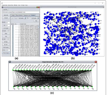
Implementation of BiClusO software
Fig. 2Implementation of BiClusOa) tabular format of biclustersb) hierarchical view of biclustersc) a single bicluster
Overlapping parameters
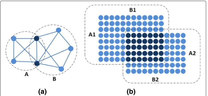
We used here two different overlapping coefficients which are 1) simple graph clus-ter overlapping coefficient and 2) biclusclus-ter overlapping coefficient. The first overlapping coefficient measures the overlapping between two clusters while applying DPClusO to the simple graph generated from the bipartite graph. IfA,Bare two simple clusters and
A∩Bbe the set of common number of nodes between them (Fig.3a) then the simple cluster overlapping coefficient is
SCov= (|A∩B|)
2
|A||B| (1)
Bicluster overlapping coefficient measures the overlapping between two biclusters. This measurement considers each bicluster as a biclique and finds the common block matrix in terms of total block area occupied by them. If the node sets of two biclusters are denoted byA1,B1 andA2,B2 (Fig.3b). The block area which denotes the number of edges in each bicluster is|A1| × |B1|and|A2| × |B2|. The common block area between two biclusters
is|A1∩A2| × |B1∩B2|. The overlapping coefficient can be expressed by the following
Equation
BCov= |A1∩A2||B1∩B2|
Fig. 3aSimple cluster overlapping coefficientbbicluster overlapping coefficient
These parameters help the user to join and filter some of the biclusters and control overlapping property of the generated bicluster set.
Computational complexity
A bipartite graph is a graph that consists of two disjoint sets of nodes,U andV, such that each edge connects a node inU with a node inV, i.e.,U andV are independent sets. Let|U| = nand|V| = mand therefore, the bipartite graph can be represented by a matrix of sizen×m. The detail of the algorithm of BiClusO is available in Karim et al. (2019). In BiClusO, calculating relation numbers betweenn(n−1)/2 pairs of the nodes of setUrequiresmn(n−1)/2 computations (Fig.1b). Therefore, the complexity for this calculation isOn2m. Similarly, the complexity for calculating Tanimito
coeffi-cient isOn2m(Fig.1d). Filtering the edges in the weighted graph and construction of a
simple graph using the threshold values of the Tanimoto coefficient and relation number needn(n−1)/2 orOn2computations (Fig.1c and d. The computational complexity for DPClusO algorithm isOn3wherenis the total number of nodes in a simple graph (Altaf-Ul-Amin et al.2012; Altaf-Ul-Amin et al.2006) (Fig.1e). If the clusters generated by DPClusO on the simple graph are of sizesp1,p2...pc, then assigning the second node set to all the clusters needsp1m,p2m....pcm=(p1+p2....pc)mcomputations. The value ofp1+p2....pcis roughly equal ton. Thus the computational complexity for assigning the second node by calculating the attachment probability isO(nm). So the total
com-putational complexity of biclustering on the first node set comprises of 1) weight graph construction using relation number and Tanimoto coefficient 2) filtering and construc-tion of simple graph 3) simple graph clustering and 4) second node attachment which is in totalO2n2m+n2+n3+nm. Similarly, the computational complexity considering the second node set isO2m2n+m2+m3+mn.
Reference methods and dataset selection
Reference BiClustering algorithms
We have chosen five other well-known biclustering algorithms namely BiMax, Plaid, xMOTIF, Spectral, And CC (Chang and Church) for performance comparison with BiClusO. These algorithms have been implemented in the R package ’biclust’ which we utilized for our experiments. BiMax recursively divides the binary data matrix using a different concentration of regions made by 1 and 0 and generates all maximal biclusters (Preli et al.2006). It can only work with binary data matrix. Plaid algorithm models the data matrices with the sum of different layers and an assumed number of biclusters. It fits the model by iteratively updating the different parameters (Lazzeroni and Owen2002). xMOTIF discretizes the data matrix by searching a set of rows following the same linear order under a set of columns to find motif (Murali and Kasif2002). Spectral algorithm uses the singular value decomposition in eigenvectors to search the coherent value over row and column where the variance is lower than a given threshold value (Yuval et al. 2003). CC uses the deterministic greedy method based on the mean square residue of a submatrix where the score is lower than a threshold (Cheng and Church2000).
Selection of dataset
We used two different types of datasets i.e. biological data and synthetic data. It is easy to compare the performance of different biclustering algorithms when the properties of the results are foreknown. Two different biological datasets are species-VOC (volatile organic compound) data and microarray gene expression data ofS. Cerevisiae. We evaluated the performance of different algorithms by measuring the statistical significance of the gen-erated biclusters in terms of biological properties. We also created synthetic dataset by embedding biclusters with different physical properties. These physical properties help us to measure the quality of the extracted biclusters by different algorithms.
Species-VOC data
The species-VOC bipartite dataset was collected from KNApSAcK (Nakamura et al.2014; Afendi et al.2011; Afendi et al.2013; Abdullah et al.2015) database. This dataset forms a sparse matrix of dimension 710 species vs. 1760 VOCs emitted by those species under different biological stress. We categorized these species under five different taxonomic levels which are kingdom, phylum, class, order, and family. Usually, similar species group under family level produce many distinct types of VOCs (Karim et al.2018). However, there are some common VOCs among such species groups.
Gene expression data
This dataset is the gene expression data of the speciesS. Cerevisiae(Brown et al.2000; Alvaro et al.2002; Lægreid et al.2003; Raghava and Han2005; Altaf-Ul-Amin et al.2014) consisting of a matrix with dimension 2644 genes vs. 79 conditions. The data point in each cell represents the logarithmic ratio of the expression levels of a particular gene under two different experimental conditions. Each column representsnlog-transformed expression-level ratios ofngenes for a single chip. We digitized the data by column-wise transformation using the following formula.
Dij=
1, Mij≥avgj+th×sdjorMij≤avgj−th×sdj.
Whereavgjandsdj represent average and standard deviation of thejthcolumn. The thresholdthis the value which determines the quantity of 1s to be set in the digital matrix. After accessing three different threshold values (th=0.5, 1 and 1.5) we considered theth
to be 1.5 which makes the digitized matrix as a sparse matrix.
Synthetic data
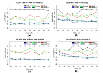
We created synthetic dataset of binary matrices using hypothetical relations between genes and conditions. We inserted a block of 1s as embedded bicluster to such matrix where 1 represents the differential expression of a gene under a condition. We changed the overlapping property and size of the biclusters and constructed four different types of such dataset: (1) equal size nonoverlapping, (ii) different size nonoverlapping, (iii) equal size overlapping and (iv) different size overlapping. Each dataset is a matrix of dimen-sion 100 genes vs. 100 conditions. Each bicluster of equal size nonoverlapping set has 10 genes and 10 conditions (Fig.4a). Different size nonoverlapping set has a varying number of genes between 5 to 10 and a varying number of conditions between 8 to 20 (Fig.4c). Each bicluster of equal size with overlapping consists of 18 genes and 18 conditions where 9 genes and 9 conditions are overlapped between biclusters (Fig.4b). Each bicluster of different size with overlapping consist of maximum 18 genes and 18 conditions with the overlapping region varying between 1 to 8 for genes and 2 to 10 for conditions (Fig.4d). We introduced noise to the non-cluster region of each dataset by randomly inserting ’1’s. Total 36 datasets were created with four types of variation and nine different noise levels from 1% to 9%.
Parameter setting
We used the default parameter setting recommended by different papers and the authors of the biclustering algorithms (Preli et al.2006; Eren et al.2012; Li et al.2012). In some cases, we slightly changed the parameters to force the algorithm to generate at least a minimum number of biclusters. For BiMax we set minimum row = 2, and minimum column=2. For Spectral we set minimum row =2, minimum column =2, maximum within variation =1, normalization = ’log’ and number of eigenvalue = 1. A high number of eigenvalue for this algorithm creates a performance issue on calculation time. The recom-mended value is 1. For xMOTIF we set sd=7, alpha=0.1, ns=10, nd=1000. For CC we set alpha=1.2, delta = .0000005. We took delta to such small value to create at least two biclus-ters. We set default parameter for Plaid algorithm of R BiClust package. For our algorithm we set CD(Cluster density)=0.5, CP=0.5(Cluster property), Tanimoto coefficient = 0.33, relation number = 5 and attachment probability = 0.5
Cluster density and Cluster property are default parameters for DPClusO algorithm. From our previous experience on some actual dataset, the optimal setting for both CD and CP is 0.5 (Eguchi et al.2018; Hossain et al.2018) which produced good results. Also user can change the cluster density between 0.5 to 0.7. Most of the cases, the actual datasets are sparse by nature. To select the best threshold on sparse matrix user can start with relation number = 2 or 3 and Tanimoto coefficient = 0.33 (Karim et al.2019). Tanimoto coefficient≥0.33 allows more than 50% similarity between 1s of two binary vectors. Very high relation number and Tanimoto coefficient might exclude some nodes from the anal-ysis (Karim et al.2019). If the data is not sparse then Tanimoto coefficient threshold can be adjusted between 0.4 to 1.0 depending on whether the required number of nodes are included in the biclusters.
Results of performance evaluation
We adopted different scoring methods to evaluate the strength of biclustering algo-rithms. The results of comparison based on different biological data and synthetic data are summarized in Figs.5,6and7. In the following we discuss in detail.
Fig. 6Performance of different algorithm based on gene expression data ofS. cerevisiae.aRanking based on BP.bRanking based on CC.cRanking based on MF
Classification of species based on VOCs
Biclustering can be used to classify species based on the VOCs they emit. We applied the hypergeometric test to the bicluster set generated from species-VOC relational data. The richness of same categorical species in a bicluster in terms of family-level taxonomy was evaluated by using the following formula
p−value=1− n−1
i=0
G i
N−G X−i
N
X
(4)
HereXis the number of species in a bicluster.Nis the number of species in the data.nis the maximum number of same categorical species belong to a specific family in a cluster.
Gis the total number of species of that category in the data. After selecting the statisti-cally significant biclusters wherep−value<=0.05, we combined the results generated by different algorithms. We created a list of clusters together with the algorithm name and their corresponding−log(p−value)in each row. We rearranged the list by descending order of−log(p−value)and therefore the top row on the list indicates the most signif-icant bicluster and the bottom row indicates the least signifsignif-icant bicluster out of all the biclusters generated by all the algorithms. In order to compare the performance of differ-ent algorithms, we selected differdiffer-ent sets of rows from the top of the list and counted the number of rows corresponding to the different algorithms within each set.
The number of biclusters generated by BiClusO, BiMax, and Spectral is more compared to other algorithms as shown in Fig.5a. Except some slightly overlapping, the BiClusO produces almost distinct biclusters. Plaid, CC and xMOTIF produce a very small num-ber of biclusters which implies that these algorithms are not suitable for finding biclusters from sparse matrices (Miranda van et al.2008). One of the limitations of BiMax is that it requires to specify the number of biclusters beforehand, otherwise produces 100 biclus-ters by default. Figure5b shows that BiClusO has the highest share among top ranking clusters based on statistical significance. Spectral biclustering shows the second best per-formance. A moderate number of the biclusters generated by Spectral has identical sets of species over different sets of VOCs.
Richness of similar function genes
Biclustering of gene expression data is expected to accumulate similar function genes in individual biclusters. In order to find the richness of similar function genes in the gene side of each bicluster, we calculated hypergeometricp-values corresponding to three different Gene Ontology (GO) terms i.e. Biological Process(BP), Cellular Component (CC), Molecular Function(MF). We used the GOstats package from R for calculating the
p−values. The result of this analysis produces a series ofp−valuerelated to different GO terms. The GO term for which thep−valueis the smallest is the most significant. For each bicluster, we selected the lowestp−valuesfor certain term under each type of ontology. The number of generated biclusters by different algorithms is different. For the sake of fair comparison, we took up to the best 50 biclusters from each algorithm. For the algorithms that produced less than 50 clusters, we took all of them. We combined the selected clusters of all algorithms corresponding to a specific ontology and sorted the clusters according to their respective−log(p−value).
According to Fig.6in all three cases of BP, CC and MF, BiClusO produces most of the best ranking biclusters among the first 30 top biclusters. In the case of BP and MF (Fig.6a and c), BiClusO clearly outperformed the other algorithms. Only in case of CC, BiMax shows almost similar performance like BiClusO (Fig. 6b). The CC (algorithm) shows the third position in all three ontology analysis. Plaid produces the smallest number of biclusters with large sizes compare with other algorithms which fail to produce good
p-value.
Comparison based on synthetic data
We evaluated the degree of similarity of bicluster sets generated by an algorithm from synthetic data by using the following matching score formula (Preli et al.2006; Eren et al.2012).
Sg(A1,B1)=
1 |A1|
(G1,C1)∈A1
max(G2,C2)∈B1
|G1∩G2|
|G1∪G2|
(5)
HereA1denotes the actual bicluster set andB1denotes the bicluster set generated by
an algorithm. An element of the bicluster setA1is denoted by(G1,C1)whereG1is the
set of genes andC1is the set of conditions. Similarly(G2,C2)denotes an element of the
bicluster setB1. The Jaccard index formula:|G1∩G2|/|G1∪G2|express the similarity
between two biclusters in terms of gene side. According to the Jaccard index, identical biclusters produce maximum value 1 whereas disjoint biclusters produce minimum value 0. The above equation finds the average of maximum matching score of each gene set fromA1to B1. Similarly, the matching scoreSc(A1,B1)was calculated considering the
matching of condition sides of biclusters. Finally the formula
S(A1,B1)=
Sg(A1,B1)×Sc(A1,B1) (6)
calculates the overall matching score from A1 to B1considering both genes and
con-ditions. If A1 be the actual bicluster set andB1 be the generated bicluster set by an
algorithm then the matching scoreS(A1,B1)represents average module recovery whereas
S(B1,A1)represents average cluster relevance (Preli et al.2006). Average module recovery
reflects the algorithm’s ability to retrieve the actual biclusters. The best case value for this score is 1 which means that all of the actual biclusters are successfully discovered by the algorithm. The number of biclusters generated by the algorithm, in this case, must be greater than or equal to the number of actual biclusters. Average cluster relevance mea-sures the similarity between generated bicluster and actual bicluster. The best case value for this score is 1 which means maximum similarity is achieved by the algorithm. The number of biclusters generated by the algorithm, in this case, must be less than or equal to the number of actual biclusters. If both scores are 1 then the algorithm successfully generates actual biclusters.
Performance on average module recovery
level increases the performance drastically degrades. Most of the cases of four types of synthetic dataset with a varied level of noises, BiClusO achieves the best results in terms of average module recovery.
Performance on average cluster relevance
Almost all of the cases of four different synthetic datasets BiClusO shows the best perfor-mance over other algorithms in terms of average cluster relevance (Fig.8). Spectral and Plaid achieve the second highest position alternatively. BiMax, xMOTIF and CC show poor performance. The Performance of BiMax is deteriorated because it produces a large number of biclusters where a substantial portion of them are dissimilar to the original bicluster set. Most of the biclusters produced by BiClusO show maximum similarity to the original bicluster set.
Conclusion
In this study, we present a GUI based implementation of our algorithm BiClusO and compare its performance with different biclustering algorithms based on two types of biological data and four types of synthetic data. Biclusters generated based on biological dataset are analyzed on the basis of statistical significance determined by Hypergeometric test in the context of taxonomical classes and different GO terms. The varying properties of size and overlapping on synthetic datasets simulate a diverse pattern of gene-condition bipartite dataset which helps to compare different algorithms effectively. The imple-mentation allows us to control the overlapping between biclusters. Also the attachment probability parameter helps to extract biclusters as bicliques. The performance of our algorithm in terms of different scoring methods on real biological datasets expresses the robustness and effectiveness of BiClusO over other algorithms. The consistency of the
performance of different algorithms to a certain degree in the case of synthetic datasets implies the correctness and significance of the comparison method we adopted in the present work. The implementation of our algorithm will be available on http://www. knapsackfamily.com/BiClusO/.
Abbreviations
BCov: Biclustering overlapping coefficient; BP: Biological process; CC (Algorithm): Biclustering algorithm; CC: Cellular component; CD: Cluster density; CP: Cluster property; GO: Gene ontology; MF: Molecular function; SCov: Simple clustering overlapping coefficient; VOC: Volatile organic compound
Acknowledgements
We are very thankful to Dr. Naoaki Ono for his cordial help and to the anonymous reviewers for their important comments.
Authors’ contributions
Md. A-U-A and MBK designed the research and conducted the experiments. SK guided the research with valuable comments. All authors have read and approved the final manuscript.
Funding
This work was supported by the Ministry of Education, Culture, Sports, Science, and Technology of Japan (16K07223 and 17K00406) and NAIST Big Data Project and was partially supported by Platform Project for Supporting Drug Discovery and Life Science Research funded by Japan Agency for Medical Research (18am0101111) and Development and the National Bioscience Database Center in Japan.
Availability of data and materials
Data is available on request from the corresponding author
Competing interests
The authors declare that they have no competing interests.
Received: 26 February 2019 Accepted: 23 July 2019
References
Abdullah AA, Altaf-Ul-Amin Md, Ono N, Sato T, Sugiura T, Morita AH, Katsuragi T, Muto A, Nishioka T, Kanaya S (2015) Development and mining of a volatile organic compound database. BioMed Res Int 2015:1–13
Afendi FM, Okada T, Yamazaki M, Hirai-Morita A, Nakamura Y, Nakamura K, Ikeda S, et al. (2011) KNApSAcK family databases: integrated metabolite–plant species databases for multifaceted plant research. Plant Cell Physiol 53(2):e1–e1 Afendi FM, Ono N, Nakamura Y, Nakamura K, Darusman LK, Kibinge N, Hirai Morita A, et al. (2013) Data mining methods
for omics and knowledge of crude medicinal plants toward big data biology. Comput Struct Biotechnol J 4(5):e201301010
Altaf-Ul-Amin Md, Katsuragi T, Sato T, Ono N, Kanaya S (2014) An unsupervised approach to predict functional relations between genes based on expression data. BioMed Res Int 2014:1–8
Altaf-Ul-Amin Md, Shinbo Y, Mihara K, Kurokawa K, Kanaya S (2006) Development and implementation of an algorithm for detection of protein complexes in large interaction networks. BMC Bioinformatics 7(1):207
Altaf-Ul-Amin Md, Tsuji H, Kurokawa K, Asahi H, Shinbo Y, Kanaya S (2006) DPClus: a density-periphery based graph clustering software mainly focused on detection of protein complexes in interaction networks. J Comput Aided Chem 7:150–156
Altaf-Ul-Amin Md, Wada M, Kanaya S (2012) Partitioning a PPI network into overlapping modules constrained by high-density and periphery tracking. ISRN Biomath 2012:1–11
Alvaro M, Dopazo J, Jansen R, Tu Y, Gerstein M, Stolovitzky G (2002) Systematic learning of gene functional classes from DNA array expression data by using multilayer perceptrons. Genome Res 12(11):1703–1715
Andrew W, Halappanavar S (2015) Application of biclustering of gene expression data and gene set enrichment analysis methods to identify potentially disease causing nanomaterials. Beilstein J Nanotechnol 6(1):2438–2448
Arindam B, Dhillon I, Ghosh J, Merugu S, Modha DS (2007) A generalized maximum entropy approach to bregman co-clustering and matrix approximation. J Mach Learn Res 8(Aug):1919–1986
Beatriz P, Giráldez R, Aguilar-Ruiz JS (2015) Biclustering on expression data: A review. J Biomed Inform 57:163–180 Bergmann S, Ihmels J, Barkai N (2003) Iterative signature algorithm for the analysis of large-scale gene expression data.
Phys Rev E 67(3):031902
Brown MPS, Grundy WN, Lin D, Cristianini N, Sugnet CW, Furey TS, Ares M, Haussler D (2000) Knowledge-based analysis of microarray gene expression data by using support vector machines. Proc Natl Acad Sci 97(1):262–267
Cheng Y, Church GM (2000) Biclustering of expression data. In: Ismb Vol. 8. pp 93–103
de Castro PAD, de França FO, Ferreira HM, Von Zuben FJ (2007) Applying biclustering to text mining: an immune-inspired approach. In: International Conference on Artificial Immune Systems. Springer, Berlin. pp 83–94
Dmitry G, Ignatov DI, Semenov A, Poelmans J (2012) Gaining insight in social networks with biclustering and triclustering. In: International conference on business informatics research. Springer, Berlin. pp 162–171
Eren K, Deveci M, Küçüktunç O, Çatalyürek ÜV (2012) A comparative analysis of biclustering algorithms for gene expression data. Brief Bioinforma 14(3):279–292
Gonçalves JP, Madeira SC, Oliveira AL (2009) Biggests: integrated environment for biclustering analysis of time series gene expression data. BMC Res Notes 2(1):124
Guojun L, Ma Q, Tang H, Paterson AH, Xu Y (2009) QUBIC: a qualitative biclustering algorithm for analyses of gene expression data. Nucleic Acids Res 37(15):e101–e101
Gurkan B, Yang J (2007) PathFinder: mining signal transduction pathway segments from protein-protein interaction networks. BMC Bioinformatics 8(1):335
Heinrich J, Seifert R, Burch M, Weiskopf D (2011) Bicluster viewer: a visualization tool for analyzing gene expression data. In: International Symposium on Visual Computing. Springer, Berlin, Heidelberg. pp 641–652
Hochreiter S, Bodenhofer U, Heusel M, Mayr A, Mitterecker A, Kasim A, Khamiakova T, et al. (2010) FABIA: factor analysis for bicluster acquisition. Bioinformatics 26(12):1520–1527
Hossain SF, Wijaya SH, Huang M, Batubara I, Kanaya S, Altaf-Ul-Amin Farhad Md (2018) Prediction of Plant-Disease Relations Based on Unani Formulas by Network Analysis. In: 2018 IEEE 18th International Conference on Bioinformatics and Bioengineering (BIBE). IEEE. pp 348–351
Kaiser S, Santamaria R, Khamiakova T, Sill M, Theron R, Quintales L, Leisch F, De Troyer E, Maintainer ORPHANED (2018) Package biclust. Title BiCluster Algoritm Version 2.0.1
Karim MB, Huang M, Naoaki ONO, Kanaya S, Altaf-Ul-Amin Md (2019) BiClusO: A novel biclustering approach and its application to species-VOC relational data. IEEE/ACM Trans Comput Biol Bioinforma.https://doi.org/10.1109/TCBB. 2019.2914901
Karim MB, Kanaya S, Altaf-Ul-Amin Md (2018) Comparison of BiClusO with Five Different Biclustering Algorithms Using Biological and Synthetic Data. In: International Conference on Complex Networks and their Applications. Springer, Cham
Karim MB, Ono N, Altaf-Ul-Amin Md, Kanaya S (2018). APBC 2018 conference, Yokohama. 15–17 January Karim MB, Wakamatsu N, Altaf-Ul-Amin Md (2017) Dedicated to Prof. T. Okada and Prof. T. Nishioka: data science in
chemistry] DPClusOST: A Software Tool for General Purpose Graph Clustering. J Comput Aided Chem 18:76–93 Lægreid A, Hvidsten TR, Midelfart H, Komorowski J, Sandvik AK (2003) Predicting gene ontology biological process from
temporal gene expression patterns. Genome Res 13(5):965–979
Lazzeroni L, Owen A (2002) Plaid models for gene expression data. Stat Sin 12:61–86
Li L, Guo Y, Wu W, Shi Y, Cheng J, Tao S (2012) A comparison and evaluation of five biclustering algorithms by quantifying goodness of biclusters for gene expression data. BioData Min 5(1):8
Miranda van U, Meuleman W, Wessels L (2008) Biclustering sparse binary genomic data. J Comput Biol 15(10):1329–1345 Murali TM, Kasif S (2002) Extracting conserved gene expression motifs from gene expression data. Pac Symp Biocomput
8:77–88
Nakamura Y, Afendi FM, Parvin AK, Ono N, Tanaka K, Morita AH, Sato T, Sugiura T, Altaf-Ul-Amin Md, Kanaya S (2014) KNApSAcK metabolite activity database for retrieving the relationships between metabolites and biological activities. Plant Cell Physiol 55(1):e7–e7
Preli A, Bleuler S, Zimmermann P, Wille A, Bühlmann P, Gruissem W, Hennig L, Thiele L, Zitzler E (2006) A systematic comparison and evaluation of biclustering methods for gene expression data. Bioinformatics 22(9):1122–1129 Qinghua H (2011) A biclustering technique for mining trading rules in stock markets. In: International Conference on
Applied Informatics and Communication. Springer, Berlin. pp 16–24
Raghava GPS, Han JH (2005) Correlation and prediction of gene expression level from amino acid and dipeptide composition of its protein. BMC Bioinformatics 6(1):59
Rui H, Madeira SC (2014) BicPAM: Pattern-based biclustering for biomedical data analysis. Algoritm Mol Biol 9(1):27 Santamaría R, Therón R, Quintales L (2014) Bicoverlapper 2.0: visual analysis for gene expression. Bioinformatics (Oxford
Engl) 30(12):1785–6.https://doi.org/10.1093/bioinformatics/btu120
Shu W, Gutell RR, Miranker DP (2007) Biclustering as a method for RNA local multiple sequence alignment. Bioinformatics 23(24):3289–3296
Streit M, Gratzl S Gillhofer, Mayr A, Mitterecker A, Hochreiter S (2014) Furby: fuzzy force-directed bicluster visualization. BMC Bioinformatics 15(Suppl 6):S4
Tanay A, Sharan R, Shamir R (2002) Discovering statistically significant biclusters in gene expression data. Bioinformatics 18(suppl):S136–S144
Yuval K, Basri R, Chang JT, Gerstein M (2003) Spectral biclustering of microarray data: coclustering genes and conditions. Genome Res 13(4):703–716
Publisher’s Note