Nov
e
l Mobile Network Service for Road Safety
J.RadhakrishnanDepartment of Computer Science, Vinayaka Missions University, Salem Tamilnadu, INDIA
Email: radhak_00@yahoo.co.in R.S.Rajesh, M.E., Ph.D
Dept. of Computer Science and Engineering, Manonmaniam Sundaranar University,Tirunelveli Tamilnadu, INDIA
Email: rs_rajesh1@yahoo.co.in
---ABSTRACT---
This paper describes a Mobile Network Service helps Road Safety Purpose. A preprocessing steps reduces the search space in a safety way. Mobile Network Service applies Safety improvement and Location tracing, a technique that focuses the optimization on critical regions. The result indicates that the Mobile Network Services reliably identifies high quality solutions.
Keywords – Collision, Fixed Stations, Location tracing, Mobile nodes, Transceiver
--- Date of Submission: 11 October 2010 Revised: 16 November 2010 Date of Acceptance: 12 January 2011 ---
I. Introduction
I
n most of the developing countries, mobile penetration is strongly correlated with economic growth and social benefits. New mobile devices, services and applications were developed. The whole computing and communication paradigms were shifted to mobile domain. The area of Mobile Computing there is considerable research work done in the field over the past one decade. There are research work on Ad hoc network protocols, communication, computing techniques such as application environment, computing methods etc., Mobile computing leads to create new awareness to researches such as Nomadic computing, pervasive computing, sensor networks etc.,The development of Mobile technology only based on communication. The mobile user has communicating with other mobile user. They are getting services from the fixed stations like railway reservation, air ticket and booking hotels etc., The social issues like Highway road information, hospital information, ambulance information, Doctors information, Police station information, location tracing of a particular place, location identification and terrorist information are not available. The limited numbers of mobile applications are available.
In these social issues, location tracking is very important concept due to the highways accident. Now a day, highway accidents are quit natural and increased the highway death. In the modern world, nobody can help the accident people. They are helpless and their accident information may reach to the Police or Ambulance in a late hours.
1.1 Accidental Deaths in India
The incidence of accidental deaths has shown a mixed trend during the decade 1995-2005 with an increase of over 32.2 percent in the year 2005 as compared to 1995. The population growth during the corresponding period was 20.4 percent whereas the increase in the rate of accidental deaths during the same period was 9.9 percent. The total of 2, 94,175 accidental deaths were reported in the country during 2005. Correspondingly, 1.6 percent increase in the population and 4.7 percent increase in the rate of Accidental Deaths were reported.
2,71,760 (92.4%) deaths were due to unnatural causes and the rest 7.6% deaths (22,415) were due to causes attributable to nature, out of total 2,94,175 accidental deaths during the year 2005.
1.2. Mobility
Mobility is the most significant feature of mobile nodes in certain applications such as cellular networks, vehicle traffic navigation systems, road safety etc., In order to model the mobility of mobile nodes, different approaches have been developed. The location information of the mobile systems is used to either verify whether mobile nodes are within the boundary of some local zone or to find out the next possible course of movement in some mobile systems. However, very little research effort has been made on extracting the location information in the presence of a node collision. Such information is very significant in the area of road safety, disaster management and similar applications where a quick and accurate location data is vital. The problem of location extraction of mobile nodes on a fixed mobile interaction frame work is taken for investigation.
mathematical concepts used in the proposed model are explained. The proposed Mobile network architecture model is described in the section four. In the fifth section, the evaluation of the proposed architecture is explained.
2. Utilities-based on authentication
The Mobile nodes and the Fixed stations (FS) having transceiver. The performance of the Transceiver is increased by the algorithm that is available in the reference “An iterative algorithm for High Performance Transceiver” [1].
The idea behind the connection between the Mobile node and FS is a New Technology for AD-Hoc interconnections between Hand-Held Terminals and Smart Objects. This technology has been found in the Literature “Micro power IR Tag – A new technology for Ad-Hoc interconnection between the Hand Held Terminals and Smart Objects” [2]. This paper prescribed in the smart object conference, France at 2003.
Almost all the systems for location tracking depend on customized hardware. A very few are systems based on software. A pure software based location tracing system is defined as WLAN (Wireless Local Area Network)
which is present in the literature “WLAN Tracker: Location Tracking and location based services in Wireless LANs” [1],[3] by Can Komar and Cem Ersoy “Wireless networking-Tele communication , Newage
The realistic mobility model is available in the paper ‘Towards Realistic Mobility Models for Mobile Ad hoc Networks’ [4]
The Shortest Path between the Mobile nodes and the FS can be calculated by using CPM technology. But some special algorithm is used in the Project [5] “Fast shortest path algorithm for Road Network and implementation” Carl eton University, Honors Project 2005, Liang Dai.
3. Mathematical Approach
Various mathematical concepts are utilized. Basically, in the mobile ad hoc network design, the network is formed as a two dimensional graph. The characteristics of the network are bounded and the boundaries are well defined. The Network paths are defined. The mobility of the mobile nodes are utilizing the mathematical queuing theory[6]. That is the entry of the mobile nodes in to the ad hoc network is Poisson distribution. Mathematically, the Fixed stations are considered as a Service channels and the service discipline as Exponential distribution.
In the mobility of the mobile nodes any collision occurs, then the shortest path between the fixed station and the mobile node is calculated using the mathematical method called critical path method.
3.1. Role of the Poisson and Exponential Distribution In queuing situation, the number of arrivals and departures (after served) during an interval of time is controlled by the following conditions.
Condition 1
The Probability of an event (arrival or departure) occurring between times t and t+h depends only on the length of h meaning that the probability does not depend on either the number of events that occur up to time t or the specific value of T.
Condition 2:
The probability of an event occurring during a very small time interval h is positive but less than 1 Condition 3:
At most one event can occur during a very small time interval h. The implication of these conditions can be studied by deriving mathematically the probability of n events occurring during a time interval t. Let Pn(t) be the probability of n events occurring during time t.
3.2. CPM - Critical Path Method
fig. 1 Network Model
4. Mobile Network Architecture Model
A model of the proposed Architecture has been designed and developed with the help of the following.
1. Basic Network Model. 2. Mobility model development 3. simulations of collision 4. POS identification 5. Path identification 6. Statistics collection 4.1. Basic Network Model
The Basic Network model consists of a Fixed Stations and the Mobile Nodes as shown in Fig. 1 In this network, the mobile nodes communicate with the Fixed Station wirelessly. These networks are extremely flexible, Self-configurable and they do not require the deployment of any infrastructure for their operation
4.1.1. Characteristics of Fixed Station
The Fixed station has a high performance transceiver. The function of transceiver is given below.
A transceiver is a combination transceiver/receiver in a single package. India radio transceiver, the receiver is silenced while transmitting. An electronic switch allows the transceiver and receiver to be connected to the same antenna and prevents the transceiver output from damaging the receiver. With a transceiver of this kind, it is impossible to receive signals while transmitting. This mode is called half duplex. Transmission and reception often but not always are done on the same frequency. Some transceivers are designed to allow reception of signals during transmission periods. This mode is known as full duplex and requires that the transceiver and receiver operate on substantially different frequencies so the transmitted signal does not interfere with reception.
Cellular and cordless telephone sets use this mode. Satellite communications networks often employ full-duplex transceivers at the surface based subscriber points. The transmitted signal is called the uplink and the received signal is called the downlink.
The transceiver transmits the fixed stations identification code to the Mobile nodes. Similarly, it receives the IP address of the Mobile node which is available in the boundary of the fixed station. That is, each fixed station has a fixed range. Within the range, the transceiver signal can be transmitted.
4.1.2. Characteristics of Mobile nodes
The Mobile nodes are moving around the fixed station range. The Transceiver in the Mobile node receives the signal from the fixed station and to transmit the IP address to the fixed station. The Mobile nodes address is allocated in the following method.
Nodes requiring global connectivity need a globally routable IP address for to avoid other solutions like network address translation (NAT). There are basically two alternatives to the issue of address allocation. They may be assigned by a centralized entity (stateful auto configuration)
or can be generated by the nodes themselves (stateless auto-configuration). In this work centralized entity can be utilized. The fixed station has the Database server.
4.2.Mobility model development
Most of the Mobility models are not realistic. The Mobile nodes are moving in a constant speed and the directions are same. The path way is straight. But in the real scenario, there are many interventions may occur when the mobile nodes moving in the path. The path way is not straight. They may curve in nature. The realistic Mobility model is available in the paper [4]. In the proposed model, the Mobility model is realistic. Since the paths are well defined, the movements of the mobile nodes are random in nature. The fixed station has a boundary to transmit the signal.
4.3.Simulations of collision
The ad hoc Network with M number of FS and ‘N’ number of mobile nodes are constructed in a simulation process. Each mobile node is assumed to have a direction, time and identification number while entering the range of FS. This information is sent to the FS, the mobile node also receives the information about the FS like the code of the FS and status as active or not. The above activities are done when the mobile node enters the FS range
The network can be simulated arbitrarily with the help of the number of mobile nodes and the FS using predefined model characteristics.
The collision is introduced at a random interval of time between the mobile nodes. The number of occurrences of collisions could be identified using various techniques. 4.4.Path Identification
When the collision occurs, then immediately the mobile nodes transceiver shorted out the fixed station identification that is available in the transceiver of the Mobile node. Using the Critical Path Method, the optimal fixed stations are identified and to send the message to that fixed stations along with the mobile nodes address and the location of the mobile node. The location of mobile node can be found with the help of identification of the mobile node, time to cross the fixed station that is already recorded in the fixed station, the current fixed station range where the mobile nodes is available and the direction of the mobile node. 5. Evaluation of Proposed Architecture
5.1. Assumptions and Notations
A mobile network model is chosen with the following set of assumptions.
each Police station and the accident location are estimated using the path finding algorithm CPM
5.2. Fixed Station Mobile Interaction
The Vehicle has a transceiver. The Fixed Station also has a Transceiver. The Vehicle cross the Police station, the Vehicle’s transceiver transmits signal to the Police station. The information has the Vehicle’s Registration number, and the Timestamp The Vehicle’s transceiver receives the Police station identification.
a) the Police station number b) Police station type
c) Police station receiver is active/not d) Time stamp
The Police station receives the Vehicle’s transceiver transmitted information such as the Vehicle’s Registration number and Timestamp. The Police station transceiver stores the information to the database. If the same Registration Number Vehicle cross the Police station then it updates the timestamp only for avoiding duplication of entry.
When Accident Occurs, immediately the Vehicle’s transceiver trace the nearest Police station by Critical Path Method (CPM).The Critical path method utilize the timestamp to arrange the Police stations according to the constraints
a) the Police station type b) the police station is active/not
The Police station transceiver receives the information about the accident Vehicle’s
(1) Registration Number (2) Timestamp
Also utilizing the Timestamp, the vehicle’s location can be determined.
5.3. Mobility Model
The ad hoc Network with one number of Police station and ‘N’ number of vehicle are constructed in a simulation process. When the vehicle crosses the Police station then the Vehicle’s transceiver is activated and it sends the signal to Police station and also receives the information about the police station.. Some times, the Vehicle may not cross the police station for various reasons like moving to some other different direction or may be in rest position or when collision occurs. Any how the information about the vehicle is recorded in the Police station server and also the information about the Police station is recorded in the vehicle.
5.4. Simulations of Collision
The network can be simulated arbitrarily with the help of the number of Vehicles and the Police stations using predefined model characteristics.
When the collision occurs, immediately the Vehicle sorts out the PS records stored in it and calculates the nearest police station with the help of CPM algorithm using
parameters as the time to cross the Police station and POS, the type of the Police station and the status of the Police station like active/inactive. This nearest Police station is hereafter called as Fittest Survival Point (FSP).
If the FSP receives the signal from the POS then FSP alerts the FSP responsibilities for immediate action to reach the POS.
After simulating the Network, the following parameters are calculated to validate the simulation process.
Maximum number of entities required for simulations is as follows.
The real time road network is shown in the Fig. 5.1 The road network starts from Tenkasi and end to Tirunelveli. The total distance from Tenkasi to Tirunelveli is 50 Kms. There are three paths are available from Tenkasi to Tirunelveli. The roads are named as SH201,SH202 and SH203. The Police stations in the road SH201 are named as SH20101 that means the first Police Station (say PS1) in the road SH201 and the second PS as SH20102 and so on. Similarly the roads SH202 and SH203 PS are named. The distance between the important towns in between Tenkasi and Tirunelveli are shown in Fig.5.1
Number of Vehicle Ni taken as 100 which is available within the starting point Tenkasi and ending point Tirunelveli, number of Police stations (PS) is taken as 10 in between Tenkasi and Tirunelveli, Range of each PS is 5 Kms, Thus the 10 PS cover an area of 50 Kms in total. Each PS can handle a maximum of one incoming vehicle at any instant and there cannot be more than 10 vehicles present at any instant. In one minute the vehicle crosses 5 Kms.
Fig.5.1. Road Network
The simulation starts with no vehicle in all 10 numbers of PS. Vehicles are induced at random interval of time with predefined speed and direction. As it progresses, it performs the registration at each PS on the path.
required to find the path to POS is calculated and tabulated. The results are graphically presented. The distribution of vehicle is changed each time. Separate set of statistics are collected for Exponential distribution and Poisson distribution.
5.4.1. Steady-State Multiple-PS Waiting Line Model With Poisson Arrivals And Exponential Service Times System
Fig.5.2. Two-PS Waiting Line
A multiple-PS waiting line consists of two or more Police Stations that are assumed to be identical in terms of service capability. In the multiple-PS system, arriving units wait in a single waiting line. To determine the steady-state operating characteristics for a multiple-PS waiting line using the formulae. These formulae are applicable if the following conditions exist.
1. The arrivals follow a Poisson probability distribution. 2. The service time for each Police station follows an exponential probability distribution.
3. The mean service rate µ is the same for each Police station.
4. The arrivals wait in a single waiting line and then move to the first Police station for service.
The following formulae can be used to compute the steady-state operating characteristics for multiple-PS waiting lines, where
λ = the mean arrival rate for the system
µ = the mean service rate for each PS k= the number of PS
The probability that no units are in the system:
0 1 0 1 (1) ( / ) ( / ) ! ! n k k n P k
n k k
λ µ λ µ µ µ λ − = = + −
∑
The average number of units in the waiting line:
0 2
(
/
)
(2)
(
1)!(
)
k q
L
P
k
k
λ µ λµ
µ λ
=
−
−
The average number of units in the system:
( 3 ) q
L L λ
µ
= +
The average time a unit spends in the waiting line:
(4)
q qL
W
λ
=
The average time a unit spends in the system:
1
(5)
qW W
µ
= +
The probability that an arriving unit has to wait for service:
0
1
(6)
!
k wk
P
P
k
k
λ
µ
µ
µ λ
=
−
The probability of n units in the system:
0 0 ( )
( / )
for
(7)
!
( / )
for
(8)
!
n n nn n k
P
P
n k
n
P
P
n k
k k
λ µ
λ µ
−=
≤
=
>
Use equations (2) through (8) for the k = 2 . For a mean arrival rate of λ = 0.2 Vehicles per second and mean service rate of µ = 0.3 Vehicles per second for each Police Station, to obtain the operating characteristics:
0
2
2
0.4815 (from Table 5.1with /
0.7)
(0.2/ 0.3) (0.2)(0.3)
(0.4815) 0.0803 vehicles
(2 1)![2(0.3) 0.2]
0.2
0.0803
0.7803 vehicles
0.3
0.0803
0.4015 sec
0.2
1
1
= W
0.4015
3.73 sec
0.3
1 0.2
2! 0.3
q q q q q WP
L
L L
L
W
W
P
λ µ
λ
µ
λ
µ
=
=
=
=
−
−
= + =
+
=
= =
=
+ =
+
=
=
22(0.3)
(0.4815) 0.1605
2(0.3) 0.2
=
−
Using equations (7) and (8), we can compute the probabilities of n Vehicles in the system. The results from these computations are summarized in Table 5.2.
Police station 1
Waiting Line
Exit vehicle Vehicle
arrival
5.4.2. Steady-States Probability of N Vehicles In The System For The Two-PS Waiting Line
In the Steady state probability of atleast 10 vehicles in the system of the two police station waiting line, the performance are tabulated in Table 5.2.
TABLE 5.1 Values of P0 for Multiple-PS Waiting Line
with Poisson Arrivals and Exponential Service Time Number of PS (k)
Ratio k=2 k=3 k=4 k=5
0.15 0.8605 0.8607 0.8607 0.8607 0.2 0.8182 0.8187 0.8187 0.8187 0.25 0.7778 0.7788 0.7788 0.7788
0.3 0.7391 0.7407 0.7408 0.7408 0.35 0.7021 0.7046 0.7047 0.7047
0.4 0.6667 0.6701 0.6703 0.6703 0.45 0.6327 0.6373 0.6376 0.6376
0.5 0.6 0.6061 0.6065 0.6065 0.55 0.5686 0.5763 0.5769 0.5769
0.6 0.5385 0.5479 0.5487 0.5488 0.65 0.5094 0.5209 0.5219 0.522
0.7 0.4815 0.4952 0.4965 0.4966 0.75 0.4545 0.4706 0.4722 0.4724
0.8 0.4286 0.4472 0.4491 0.4493 0.85 0.4035 0.4248 0.4271 0.4274
0.9 0.3793 0.4035 0.4062 0.4065 0.95 0.3559 0.3831 0.3863 0.3867
1 0.3333 0.3636 0.3673 0.3678 1.2 0.25 0.2941 0.3002 0.3011 1.4 0.1765 0.236 0.2449 0.2463 1.6 0.1111 0.1872 0.1993 0.2014 1.8 0.0526 0.146 0.1616 0.1646 2 0.1111 0.1304 0.1343
TABLE 5.2 Steady-State Probability of n Vehicles in the System for the Two-PS Waiting Line
POISSON ARRIVAL
Arrival 10 per min
Mean arrival 0.2 per sec
λ 0.2
No. of Arrivals Probability
0 P0 0.8187
1 P1 0.1637
2 P2 0.0164
3 P3 0.0011
4 P4 0.0001
5 P5 0
Where P0 , P1 , P2 , P3 , P4 , P5 are the Poisson arrival
with probability of 0,1,2,3,4 and 5 arrivals respectively, which are calculated directly from the formula (7) and (8).
EXPONENTIAL
Service 20 per min
Mean 20/60 per sec
µ 0.3 per sec
Probability service time <=0.5 sec 0.3935
service time <=1 sec 0.6321
service time <=2 sec 0.8647
Data Description Entry
Number of Police Stations 2
Service rate (per Police station per sec) 0.3 Vehicles arrival rate {per sec} 0.2 Queue capacity (maximum waiting space) M
Vehicles number M
with the output being:
Vehicles arrival rate (λ) per sec
0.2
Service rate per PS (µ) per sec
0.3
λ/µ 0.7 Probability of all PS are idle Po 0.4815
Average number of vehicles in the queue
Lq 0.0803 vehicles
Average number of vehicles in the system
Ls 0.7803 vehicles
Average time mobile nodes spends in the queue
Wq 0.40 sec
Average time mobile nodes spends in the system
Ws 3.73 sec
The Value of Po is taken from the TABLE 5.1. The
values of Lq, Ls, Wq and Ws are calculated using the
equations (2) through (5).
The various Police stations in between Tenkasi and Tirunelveli road network Fig.5.1 records are listed below.
TABLE 5.3 Police Station Record
PS VEHICLE ENTRY TIME
SH20101 MB1 2:05:06 PM
SH20101 MB2 1:39:59 PM
SH20101 MB3 2:02:05 PM
SH20101 MB3 2:02:09 PM
SH20102 MB1 1:40:00 PM
SH20103 MB1 1:40:02 PM
SH20104 MB2 1:40:03 PM
SH20108 MB1 1:58:46 PM
/
SH20202 MB2 1:40:00 PM
SH20203 MB2 2:04:47 PM
SH20203 MB2 2:05:08 PM
SH20204 MB2 2:05:10 PM
SH20205 MB2 2:05:11 PM
SH20206 MB2 2:05:13 PM
SH20207 MB2 2:05:14 PM
SH20304 MB2 1:40:06 PM
SH20304 MB3 2:05:10 PM
SH20305 MB3 2:05:10 PM
SH20306 MB3 2:05:11 PM
SH20307 MB3 2:05:12 PM
In the above Police station record, it is observed that in the PS namely SH20101 having the records of vehicles namely MB1,MB2 and MB3 and so on.
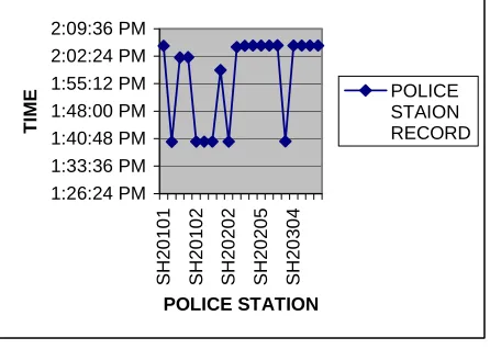
From the above records the number of vehicles available in a particular police station at a particular time is viewed in a Fig. 5.3.
1:26:24 PM 1:33:36 PM 1:40:48 PM 1:48:00 PM 1:55:12 PM 2:02:24 PM 2:09:36 PM
SH20
10
1
SH20
10
2
SH20
20
2
SH20
20
5
SH20
30
4
POLICE STATION
TI
ME
POLICE STAION RECORD
Fig.5.3 Police Station Record
The available vehicles in the road network records are listed in the Table 5.4
TABLE 5.4 Vehicle Record
PS VEHICLE TYPE STATUS ENTRY
TIME
SH20101 MB1 PS Y 2:05:06 PM
SH20101 MB2 PS Y 1:39:59 PM
SH20101 MB3 PS Y 2:02:05 PM
SH20101 MB3 PS Y 2:02:09 PM
SH20102 MB1 PS Y 1:40:00 PM
SH20103 MB1 PS Y 1:40:02 PM
SH20104 MB2 PS Y 1:40:03 PM
SH20108 MB1 PS Y 1:58:46 PM
SH20202 MB2 PS Y 1:40:00 PM
SH20203 MB2 PS Y 2:04:47 PM
SH20203 MB2 PS Y 2:05:08 PM
SH20204 MB2 PS Y 2:05:10 PM
SH20205 MB2 PS Y 2:05:11 PM
SH20206 MB2 PS Y 2:05:13 PM
SH20207 MB2 PS Y 2:05:14 PM
SH20304 MB2 PS Y 1:40:06 PM
SH20304 MB3 PS Y 2:05:10 PM
SH20305 MB3 PS Y 2:05:10 PM
SH20306 MB3 PS Y 2:05:11 PM
SH20307 MB3 PS Y 2:05:12 PM
From this Table 5.4, the Vehicle MB1 having the record of Police stations SH20101, SH20102, SH20103, SH20108. The status ‘Y’ identifies that the Police station is Active. ie the Police station transceiver responses the vehicle’s signal.
Using the Table 5.4, the vehicle records are viewed graphically in Fig.5.4
1:26:24 PM 1:55:12 PM 2:24:00 PMTime
VEHICLE
Fig 5.4. Vehicle Record 5.5. Collision Point (POS)
When the Vehicles are moving along any direction and any path, the collision may occur then the vehicle records having the Police stations information. This Police stations and the Vehicle’s path are viewed in Fig. 5.5.
Fig.5.5. Vehicle moving Path
From that Fig.5.5., it is observed that there are three paths available from Tenkasi to Tirunelveli. POS is the accident location. The direct line is the accident vehicle’s moved path
TABLE 5.5 Accident Vehicle Record
PS VEHICLE TYPE STATUS
ENTRY TIME
EXIT
TIME DURATION
SH20101 MB2 PS Y
1:39:59 PM
1:40:00
PM 1
SH20202 MB2 PS Y
1:40:00 PM
1:40:02
PM 2
SH20203 MB2 PS Y
1:40:02 PM
1:40:03
PM 1
SH20104 MB2 PS Y
1:40:03 PM
1:40:05
PM 2
SH20204 MB2 PS Y
1:40:05 PM
1:40:06
PM 1
SH20304 MB2 PS Y
1:40:06 PM
1:40:07
PM 1
The vehicle namely MB2 is the accident vehicle. Whose record is displayed in the Table 5.5. The vehicle MB2 enter the boundary of the PS SH20101 in the time 1:39:59 PM and the exit the Boundary by 1:40:00 PM. So the time duration to cross this boundary to next is 1 sec. Similarly for the other records of the vehicle MB2.
From the accident vehicle records, the Police stations which are crossed during the particular time duration is graphically represented in the Fig.5.6
Fig. 5.6. Accident Vehicle Duration
From the Table 5.5, the Accident Vehicle MB2 travel through the Police stations SH20101, SH20104, SH20202, SH20203, SH20204, SH20304 are tabulated
PS
SH 20101
SH 20101
SH 20101
SH 20202
SH 20203
SH 20104
SH 20304
SH 20204
SH 20202
SH 20104
SH 20304
SH 20203
SH 20204
SH 20204
SH
20204 POS
From the Table 5.5, the Accident Vehicle MB2 travel through the Police stations SH20101,SH20104,
SH20202, SH20203, SH20204, SH20304 in the following time intervals.
PS
SH 20101
SH 20101
SH 20101
SH 20202
SH 20203
SH 20104
SH 20304
SH 20204
SH 20202
SH 20104
SH 20304
SH 20203
SH 20204
SH 20204
SH
20204 POS
Time (sec)
1 0 0 2 1 2 1 1 From the above Table, it is observed that there is no direct path between the Police Stations SH20101 and SH20104. Similarly there is no direct path between the Police stations SH20101 and SH20304.. Also the time duration of the vehicle MB2 moves from PS SH20101 to SH20202 is 1 sec and so on.
The collision spot that is POS can be identified using Critical path method as follows
5.6. Path Identification
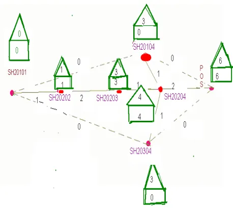
The path can be identified and the shortest path can be found using Critical Path Method. The path map is shown in Fig.5.7
Fig. 5.7. Vehicle Path Map by CPM Initialization
Step 0: Place Police station SH20101 at the beginning of the Police station .Place a POS at the end of the network. Place an ES flag value of zero on the designated origin PS, and let EF(1) = d(1) for the first PS (where the duration of both SH20101 and POS is taken to be zero).
0 0.2 0.4 0.6 0.8 1 1.2 1.4 1.6 1.8 2
Du
ra
ti
o
n
1 2 3 4 5 6
Forward Pass
Step 1: Pick any PS of Fig.5.7 such that all of its predecessors have EF time flags. If none remain, i.e. the last POS has just been flagged, go to the Backward Pass. Step 2: Let the ES(k) time for the selected PS be the maximum of the EF times at the preceding PS, and set the EF(k) time for PS equal to ES(k) + d(k). Return to step 1. Utilizing the following formulae for the early start and finish time can be calculated and displayed in the Fig.5.7.
Assume SH20101,SH20202, SH20104, SH20304, SH20203, SH20204, POS are A,B,C,D,E,F,G respectively. Task A: ESA =0
Task B: ESB = Max(ESA+tA)=1
Task C: ESC = Max(ESA+tA)=0
Task D: ESD = Max(ESA+tA)=0
Task E: ESE = Max(ESB+tB)=3
Task F: ESF = Max(ESB+tB, ESC+tC1 ,ESD+ tD1 )=4
Task G: ESG = Max(ESF+tF, ESC+tC2 ,ESD+ tD2 )=6
Backward Pass
Initialization: Set the LF time at the POS equal to the EF time, so that no delays at the final time are allowed. Then set the LS there equal to the ES, as well. Hence the PS slack at the last PS is zero.
Step 3. Choose any PS such that all following PS have LS time flags. If none remain, i.e. the beginning of the PS has just been flagged, go to the computation of slacks.
Step 4. Set the LF(j) time for the selected PS to the minimum of the LS times at the succeeding PS, and set the LS(j) time for PS equal to LF(j) - d(j). Return to step 3. Utilizing the following formulae for the late start and finish times can be calculated:
Task G: LFG =6
Task F : LFF=Min(LFG-tF)=4
Task C : LFC=Min(LFG-tC1, LFF-tC2)=3
Task D : LFC=Min(LFG-tD1, LFF-tD2)=3
Task E : LFE=Min(LFF-tE)=3
Task B : LFB=Min(LFE-tB)=1
Task A : LFC=Min(LFB-tA1, LFC-tA2, LFD-tA3)=1
Activity Slacks
Let activity slack S(k) = LS(k) - ES(k) for each PS. Activities with zero slack are called critical activities, and are always found on one or more critical paths. Here only one path is Critical. The minimum duration can be calculated and tabulated in the Table 5.6. The Fig.5.7
seems to be very clearly viewed the critical path and time duration.
TABLE 5.6 Shortest path calculation using CPM
PS
SH 20101
SH 20101
SH 20101
SH 20202
SH 20203
SH 20104
SH 20304
SH 20204
SH 20202
SH 20104
SH 20304
SH 20203
SH 20204
SH 20204
SH 20204 POS
Time (sec)
1 0 0 2 1 2 1 1
Path Duration
1 0 0 1 1 0 0 1 6
A B E F Critical
From the Table 5.6 , it tells that the accident vehicle MB2 cross the Police stations SH20101 and the Police station SH20202. The time duration to cross the boundary SH20101 to SH20202 is 1sec. Similarly from SH20202 to SJ20203 and the time duration is 2sec and from SJ20203 to SH20204 and the time duration is 1 sec. Also to cross from SH20204 to POS and the time duration is 1 sec. There is no direct path from SH20101 to SH20104 ,there is no direct path from SH20101 to SH20304 and there is no direct path from SH20104 to SH20204. Also there is no direct path from SH20304 to SH20204. In the Table 5.6. , if the path available then it can be coded as ‘1’ else ‘0’
It revels that there is only one Critical Path available. Ie. from SH20101 to SH20202 , from SH20202 to SH20203, from SH20203 to SH20204 and from SH20204 to POS.
ie. A->B->E->F
This path is optimum one; the maximum time duration is 6 seconds.
. The Accident vehicle’s transceiver transmits the signal to Fittest Survival point (FSP), i.e. the Police station SH20204.
Since it is the nearest PS. If it is not responded then transmit the signal to the second FSP SH20203 (ie next to nearest PS). If it is also not responded then transmit the signal to the third FSP SH20202 and similarly SH20101.
5.6. Conclusion
vehicle’s transceiver having only limited number of Police station addresses especially the last crossed police stations address only.
This Proposed frame work can be utilized for High way thefts and traffic intensity at an important locations and Ambulance services etc.,
REFERENCES
[1] Asoke K Talumkder, Roopa R Yuvagal. Mobile Computing (1st Edition. TATA McGraw- Hill Publishing Company Ltd., New Delhi, 2006).
[2] Chris Johnson. First workshop on Human Computer interaction with Mobile devices, Department of Computer science, University of Glasghow,Scotland,1999
[3]Uyless Black, Computer Networking (Second Edition. Prentice Hall of India, New Delhi, 2002)
[4] Amit Jardosh, Elizabeth M. Beilding-Royer, Kevin C.Almeroth, Subhash Suri, Towards Realistic Mobility Models for Mobile Ad hoc Networks. University of California at Santa Barbara.2002
[5] Liang Dai ,Fast Shortest path algorithm for Road Network and implementation, Carleton University,2005 [6] Hamdy A.TAHA, Operations Research (2nd Edition Mac Millan Publishing Co., Inc.1985)
[7] Geoferry Gardon, System simulation (2nd Edition, Prentice Hall of India Pvt. Ltd., New Delhi.1989)
[8]Mario Dorigo,Luca marin Gambar della . Ant colonies for the Traveling Salesman Problem. page 1-5 University Libre de Bruxselles, Belgium,2001
[9] Richard Baraniuk, Edward Knightly. Edge-based Traffic processing and service inference for high-performance networks. page 1-3 RICE university, Taiwan,2004
[10] G.H. Forman and J. Zahorjan. Chellanges of Mobile Computing. IEEE Computer, 27(4):page38-47,April,1994 [11] A.Jones. Mobile Computing to Go. IEEE Concorrency,7(2):page22,23 April to June, 1999.
[12]A.Krikelis. Location- dependent Multimedia
computing. IEEE concurrency. 7(2): 13 to 15 April to June .1999.
Authors Biography
Radhakrishnan has completed M.Sc., at Aditarnar College of Arts and Science,
Tiruchendur and five years experience as a Lecturer in Computer Science department, Aditanar College of Arts and Science, Tiruchendur. Now doing Ph.D in Computer Science at Vinayaka Missions University, Salem. Presently working as an Assistant Programmer at Tenkasi Municipality. Very much interested to develop Applications of Mobile Network Models.