In Honour of Distinguished Professor Dr. Mir Masoom Ali On the Occasion of his 75th Birthday Anniversary PJSOR, Vol. 8, No. 3, pages 655-667, July 2012
Prediction of Rainfall Using Logistic Regression
A.H.M. Rahmatullah Imon
Department of Mathematical Sciences Ball State University, Muncie, IN 47306 USA
Manos C Roy
Department of Statistics
University of Rajshahi, Rajshahi-6205 Bangladesh
S. K. Bhattacharjee Department of Statistics
University of Rajshahi, Rajshahi-6205 Bangladesh
Abstract
The use of logistic regression modeling has exploded during the past decade for prediction and forecasting. From its original acceptance in epidemiologic research, the method is now commonly employed in almost all branches of knowledge. Rainfall is one of the most important phenomena of climate system. It is well known that the variability and intensity of rainfall act on natural, agricultural, human and even total biological system. So it is essential to be able to predict rainfall by finding out the appropriate predictors. In this paper an attempt has been made to use logistic regression for predicting rainfall. It is evident that the climatic data are often subjected to gross recording errors though this problem often goes unnoticed to the analysts. In this paper we have used very recent screening methods to check and correct the climatic data that we use in our study. We have used fourteen years’ daily rainfall data to formulate our model. Then we use two years’ observed daily rainfall data treating them as future data for the cross validation of our model. Our findings clearly show that if we are able to choose appropriate predictors for rainfall, logistic regression model can predict the rainfall very efficiently.
Keywords and Phrases: Rainfall,Climatic Variables, Spurious Observations, Outliers,
Logistic Regression, Generalized Standardized Pearson Residuals, Cross Validation, Cohen’s Kappa, Misclassification.
1. Introduction
makers for a reliable prediction of rainfall. Therefore it is really very important to be able to predict rainfall correctly.
A variety of approaches have been employed in the literature (see Ahmed and Karmakar, 1993; Salinger and Griffiths, 2001) to predict rainfall. Most of the methods were based on linear models and the findings were inconclusive. Moreover, they lack diagnostic checking which has become an essential part of data analysis. In this paper we employ the logistic regression technique to predict rainfall. In recent times, this method is commonly employed in many fields including biomedical research, business and finance, criminology, ecology, engineering, health policy, linguistics, wildlife biology etc. Logistic regression is useful for situations in which we want to be able to predict the presence or absence of an outcome (e.g, rainfall) based on values of a set of predictor variables. In our study we have used a climatic data set from Bihar, India, that has been extensively analyzed by many others (Mollaet al., 2006). Although climatic data are usually subjected to gross measurement error, we often see that this issue is not much focused in the literature. Before fitting the model by a logistic regression, we use some recently developed data screening methods like brushing and clustering to identify spurious observations. After fitting the model we employ some recently developed logistic regression diagnostics like Generalized Standardized Pearson Residuals (Imon and Hadi, 2008) to identify the outliers. Then we apply the cross validation technique which is a very popular and useful technique (Montgomeryet al. 2006; Rao, 2005) for the validation of the fitted model for the future data. We measure the probability of misclassification error since the response in our study is a class variable. We also use Cohen’s Kappa (Cohen, 1960) statistic to test the concordance of rainfall by the logistic regression model.
2. Data and Methodology
In our study we have used the daily rainfall data for adjoining areas in Giridhi, Bihar, India that are collected from the Indian Statistical Institute (ISI) Kolkata database. Climatologically the area under the study is located in the tropical Indian monsoon region. The climate of the area before the monsoon is characterized by a hot summer season, which is called the pre-monsoon season. However in early March, the area also experiences significant rainfall and that continue until August. The data set contain daily rainfall update for the period 1989 to 2004 together with some other climatic variables, such as evaporation (mm), maximum temperature (
c
), minimum temperature (
c
), humidity at 8:30 am (%) and humidity at 4:30 pm (%) which are believed to be important predictors for rainfall.2.1. Checking of Data
necessarily ‘bad’ or ‘erroneous’, and the experimenter may be tempted in some situations not to reject an outlier but to welcome it as an indication of some unexpectedly useful industrial treatment or surprisingly successful agricultural variety.This type of outliers may come as an inherent feature of the data. Sometimes outlier might occur because of an execution error mainly due to an imperfect collection of data. We may inadvertently choose a biased sample or include individuals not truly representative of the population we aimed to sample. But sometimes outliers might occur due to gross measurement error. Observations arising from large variation of the inherent type are called outliers, while observations subjected to large measurement or execution error are termed spurious observations (Anscombe and Guttman, 1960). There are many different ways of handling outliers, but in case of spurious observation we need to correct the observations (if possible) or delete them (if correction is not possible) from the further analysis.
A large body of literature is now available regarding how to identify outliers (see Barnett and Lewis, 1994; Huber 2004). But in our study we try to locate the spurious observations first. These are the observations which contain some impossible values and index plot, scatter plot or 3D plot of variables can often locate them clearly. Analytically we can apply a variety of clustering methods (see He et al., 2003) and observations forming a very unusual cluster(s) may be considered as spurious observations. However, in our study we have used clustering techniques available in S-Plus that are developed by Struyf et al. (1997).
2.2. Logistic Regression
Logistic regression allows one to predict a discrete outcome, such as whether it will rain today or not, from a set of variables that may be continuous, discrete, dichotomous, or a mix of any of these. Generally, the dependent or response variable is dichotomous, such as presence/absence or success/failure, i.e., the dependent variable can take the value 0 or 1 with a probability of failure or success. This type of variable is called a Bernoulli (or binary) variable. Although not as common and not discussed in this paper, applications of logistic regression have also been extended to cases where the dependent variable is of more than two cases, known as multinomial or polytomous regression.
Consider a simplekvariable regression model
wherek=p+ 1. We would logically let
Generally, where the response variable is binary, there is considerable empirical evidence indicating that the shape of the response function should be nonlinear (in variable). A monotonically increasing (or decreasing) S –shaped (or reversedS –shaped) curve could be a better choice. We can obtain this kind of curve if we choose the specific form of the function as
where .
p pX
X X
Y
E( | )0 1 1...
stic. characteri that
possess does
unit th -i the if 1
stic characteri the
have not does unit th -i the if 0
i y
Z Z X
exp exp
1
This function is called the logistic response function. HereZ is called the linear predictor defined by
Z=
The model in terms ofYwould be written as
It is a well-known problem that the binary response model violates a number of ordinary least squares (OLS) assumptions. Hence it is a common practice to use the maximum likelihood (ML) method based on iterative reweighted least squares (IRLS) algorithm. In linear regression R2 is a very popular diagnostic for testing the goodness of fit. But in
logistic regression R2 is not usually recommended because of its well-known disadvantage
of possessing very low values. One can use adjusted R2 which is also known as
NagelkerkeR2 in the literature. Perhaps the deviance statistic is a better option for testing
the goodness-of-fit in logistic regression which corresponds to the error sum of squares (SSE) in linear regression. Deviance is the difference between observed likelihood and expected likelihood. It is used in logistic regression for statistical inference. We know the asymptotic property of likelihood ratio statistic lis demonstrated by-2 lnl ~ . Here we define the deviance statistic asD= -2 lnland its value is generally compared with the value of chi-square with n – k degrees of freedom. For grouped data we use commonly use the goodness-of-fit technique suggested by Hosmer and Lemeshow (2000). The Hosmer-Lemeshow statistic is given by
where gdenotes the number of groups, nj is the number of observation in the j-th group,
j
O is the sum of theYvalues for thej-th group, and ˆj is the average probability for thej
-th group. It is interesting to note -that -the statistic C differs slightly from the usual chi-squared goodness-of-fit test, as the denominator in above expression is not the expected frequency. Rather, it is the expected frequency for the j-th group multiplied times one minus the average of the estimated probabilities for the j-th group. Thus each of the g
denominators will be less than thegexpected frequencies, and there will be a considerable difference when ˆj is close to 1. In our study we use both the deviance and the
Hosmer-Lemeshow statistic for the adequacy of model fitting.
In linear regressiont–statistics are used in assessing the value of individual regressors when other regressors are in the model. In logistic regression we generally use the statistic
W =
which is called the Wald statistic. It should be noted thatWdoes not have at–distribution, even though it does have the same form as a t statistic. Rather, it is assumed that
Wisasymptotically normal.
X XY
E( | )
2
k n
g
j j j j
j j j
n n O C
1
2
1
ˆ ˆ
ˆ
i i es
ˆ . .
ˆ
2.3. Identification of Outliers in Logistic Regression
In recent time diagnostic has become an essential part of logistic regression. The rationale for diagnostics is mainly the identification of outliers, which are the ill-fitted covariates in the model. Let denote the vector of estimated coefficients. Thus the fitted values for the logistic regression model are
We define thei-th residualas
, i= 1, 2, ... ,n
Regression residuals are often expressed in terms of the hat matrix and they form basis of many diagnostics. Pregibon (1981) derived a linear approximation to the fitted values, which yields a hat matrix for logistic regression as
whereVis annndiagonal matrix with general element . The diagonal elements ofHare called the leverage values. In logistic regression, the residuals measure the extent of ill-fitted factor/covariate patterns. Hence the observations possessing large residuals are suspect outliers. The Pearson residual for thei-th observation is given by
, i= 1, 2, …,n
If we use the Pregibon (1981) linear regression-like approximation for the residual for the
i-th observation, we obtain
The above approximation helps us to define the Standardized Pearson residuals (SPR) given by
, i= 1, 2, …,n
We call an observation outlier, if its corresponding Pearson residual or standardized Pearson residual exceeds 3 in absolute term.
Like the linear regression, the logistic regression also suffers from masking (false negative) and swamping (false positive) problems when a group of outliers are present in the data. A number of diagnostics procedures have been suggested to identify multiple outliers in linear regression (Barnett and Lewis, 1993; Montgomeryet al., 2001), but this issue is not much addressed in logistic regression. When a group of observations indexed by D is omitted, let be the corresponding vector of estimated coefficients. Thus the corresponding fitted values for the logistic regression model are
When a group of observationsD is omitted, we define deletion weights for the entire data set as
,i= 1, 2, …,n
ˆ
X yi ˆiˆ
i i i y ˆ
ˆ
1 12 2 1 XV VX X X VH T
i
i
ˆ 1ˆ
i R R T R T i Di x X V X x
b 1
T D
i D T i D i x x ˆ exp ˆ exp ˆ 1
D
ˆ i i i i v yr ˆ
i vi hi
V ˆ 1
i
It should be noted that is thei-th diagonal element of . We also define
and
Using the above results and also using the linear-regression like approximation, Imon and Hadi (2008) define thei-th Generalized Standardized Pearson Residual (GSPR), based on a robust fit of the model, as
We call an observation outlier if its corresponding GSPR exceeds 3 in absolute term.
2.4. Cross Validation
Since the fit of the regression model to the available data forms the basis for many of the techniques used in the model development process, it is tempting to conclude that a model that fits the present data well will also be successful in fitting the future data. But this is not necessarily so. Hence before the model is released to the user, some assessment of its validity is should be made.
According to Montgomeryet al. (2006), three types of procedures are useful for validating a regression model. (i) Analysis of the model coefficients and predicted values including comparisons with prior experience, physical theory, and other analytical models or simulation results, (ii) Collection of new data with which to investigate the model’s predictive performance, (iii) Data splitting, that is, setting aside some of the original data and using these observations to investigate the model’s predictive performance. Since we have a large number of data set, we prefer the data splitting technique for cross-validation of the fitted model. In data splitting technique we can take subset that contains 80 to 90% of the original data (see Rao, 2005), develop a prediction equation using the selected data, and apply this equation to the samples set aside. These actual and predicted output (for the samples set aside) help us to compute the mean squared error if the response variable is quantitative or misclassification probability if the response is class variable.
2.5. Cohen’s Kappa
We have just mentioned that misclassification probability from the cross validation analysis could be an indicator of the validity of the model. For example, a misclassification probability less than 5 to 10% would tell that the model is valid for the future observations as well. But perhaps a better option is to use Cohen’s kappa (Cohen 1960) statistic which is generally a robust measure of concordance for dichotomous data. It was originally devised as a measure of ‘inter-rater’ agreement, for assessments using psychometric scales, but it serves well for the likes of presence-absence data and it is also very popular to the statisticians (see McBride, 2005) after so many years of its origination. To compute this coefficient we have to calculate the expected frequencies of each cell of a contingency table exactly in a similar way that we do for the chi-square test for the association. When we
D i
b
TR R T
R V X X
X
X 1
D
i D i D iv ˆ ˆ
1 D
i D i D
i v b
h
havenobservations and
r
i i
a 1
is the number of agreed objects in anrrcontingency table,
Cohen’s Kappa is obtained as
r
i i r
i i r
i i
e n
e a
1
whereei is the expected cell frequencies corresponding to the agreed classes. Obviously
lies between 0 and 1 and a high value of (say 0.6 or more) indicates that the agreement is good (see Landis and Koch, 1977).
3. Results and Discussion
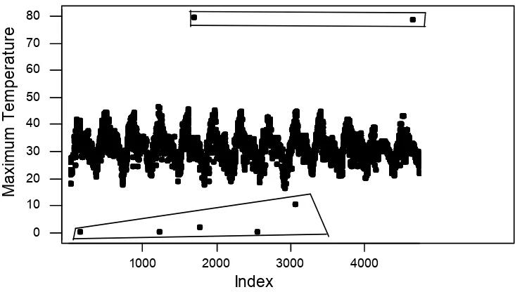
In this section we analyzed our data. Although all the weather parameters for this data were measured with the instruments specified by Indian Meteorological Department, Government of India and this data set has been analyzed extensively by many authors (see Mollaet al., 2006), we check the data for possible spurious observations before any formal analysis. At first we consider the time series (TS) plot of the maximum temperature as given in Figure 1.
4000 3000
2000 1000
80
70 60 50 40
30 20 10
0
Index
M
axi
m
um
T
em
pe
ra
tu
re
Figure 1: TS plot of maximum temperature (
c
)4000 3000
2000 1000
100 90 80 70 60 50 40 30 20 10 0
Index
M
in
im
um
T
em
pe
ra
tu
re
Figure 2: TS plot of minimum temperature (
c
)We observe more unrealistic scenario when we plot the minimum temperature data as shown in Figure 2. There is absolutely no point in favour of saying that the minimum temperature in Bihar even in a hot summer day could rise up to 95
c
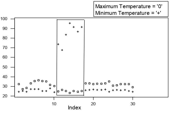
. S-Plus separates another group of spurious observation in this regard.10 20 30
20 30 40 50 60 70 80 90 100
Index
Maximum Temperature = '0' Minimum Temperature = '+'
Figure 3 presents a TS plot of daily maximum and minimum temperatures on a same graph. Here the maximum temperature is plotted as 'o' and the minimum temperature is marked by '+'. Since we have a large number of observations, the TS plot using all data looks a bit messy. To get a better view, we use the 'brushing' command of S-Plus to select a portion of data where this irregularity is more clearly visible.
The existence of spurious observations in the Climatic data of Bihar is very clear from Figure 3. Perhaps one can argue in favour of very high or very low maximum and/or minimum temperatures, but it is simply impossible that in a same day the recorded minimum temperature can be more than the maximum temperature. This gross recording error did not happen only once, but it happened in several consecutive days.
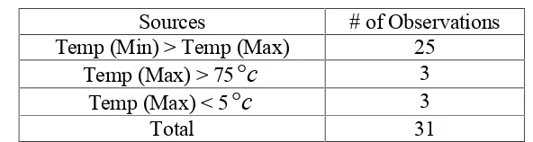
Although we anticipated that the Climatic data of Bihar possess a good quality, we see in several occasions the existence of gross measurement or recording error. So we feel to correct the data before further analysis. We employ the clustering technique that is available in S-Plus to find very bad clusters and the results are presented in Table 1.
Table 1:Spurious Observations in Bihar Climatic Data
Sources # of Observations
Temp (Min) > Temp (Max) 25
Temp (Max) > 75
c
3Temp (Max) < 5
c
3Total 31
The original climatic data of Bihar contain 5606 observations, which are the daily data, measured over a period of 16 years (1989 to 2004). After a very careful investigation we locate 31 observations as spurious because they are subjected to gross measurement error. Here the percentage of spurious observations is about 0.55%. However, we must mention that we have used the clustering technique very loosely here just to identify very bad clusters. That does not erase the possibility of the existence of few more outliers in the data. Since we would check for outliers in the process of model fitting later on, we just skip the issue for the moment. After the detection of spurious observations, the immediate question comes to our mind, what we should do with them. We can treat the spurious observations as missing data. There are a number of methods for estimating the missing data but for this particular data since the sample size is large, we would follow Samad and Harp (1992) discarding the spurious observations from the data set.
Table 2: Logistic Regression Table
Predictor Coefficient Standard Error Wald Statistic P- value Odds Ratio
Constant -6.8583 0.51591 -13.29 0.000
Evaporation -0.2594 0.02864 -9.06 0.000 0.77
Temperature (Max) 0.0455 0.01200 3.79 0.000 1.05
Temperature (Min) 0.0617 0.00759 8.13 0.000 1.06
Morning Humidity -0.0152 0.00499 -3.04 0.002 0.98
Afternoon Humidity 0.0593 0.00409 14.50 0.000 1.06
Table 3:Goodness-of-Fit Tests
Method Statistic Degrees of Freedom p– value
Deviance 3636.42 4921 1.000
Hosmer-Lemeshow 13.69 8 0.090
We observe from the results presented in Table 2 that all the predictors we consider in the model have significant impacts in the fitting of the model. Maximum and Minimum temperatures and afternoon humidity have positive effects on rainfall while the effects of evaporation and morning humidity are negative. Meteorologists generally believe that maximum temperature should have negative impact on the rainfall, but we get a result that is somewhat different. The deviance statistic shows (see Table 3) that the data adequately fit the model but the Hosmer-Lemeshow statistic shows that the fit is not good at the 10% level of significance.
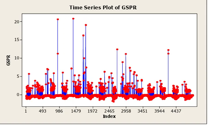
Now we employ a diagnostic to check whether there is any outlier in the data. We use the Generalized Standardized Pearson residuals (GSPR) suggested by Imon and Hadi (2008) in this regard. We observe from the index plot of GSPR (see Figure 4) that a number of outliers are present in this data. Numerical results suggests (it is not shown for brevity) that 84 observations (1.70% of the total data) had there GSPR values greater than 3 in absolute terms.
Index
GS
PR
4437 3944 3451 2958 2465 1972 1479 986 493 1 20
15
10
5
0
Time Series Plot of GSPR
To investigate the impact of the outliers we omit them from the data and fit the logistic regression model once again with the rest of the data. The revised results are presented in Tables 4 and 5.
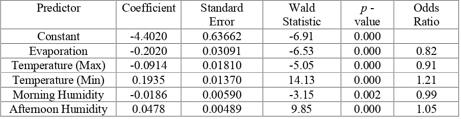
Table 4: Logistic Regression Table without Outliers
Predictor Coefficient Standard
Error StatisticWald valuep- OddsRatio
Constant -4.4020 0.63662 -6.91 0.000
Evaporation -0.2020 0.03091 -6.53 0.000 0.82
Temperature (Max) -0.0914 0.01810 -5.05 0.000 0.91
Temperature (Min) 0.1935 0.01370 14.13 0.000 1.21
Morning Humidity -0.0186 0.00590 -3.15 0.002 0.99
Afternoon Humidity 0.0478 0.00489 9.85 0.000 1.05
The results presented in Table 4 shows that all the predictors we consider in the model have significant impacts in the fitting of the model. Minimum temperatures and afternoon humidity have positive effects on rainfall while the effects of maximum temperature, evaporation and morning humidity are negative. These results makes more sense than the results we obtained earlier as we now see that the maximum temperature is having a negative effect on rainfall as anticipated. We also see from the Hosmer-Lemeshow statistic that a significant improvement in the fitting of the model has been achieved (p – value increased from 0.09 to 0.67) after dropping the outlying cases.
Table 5: Goodness-of-Fit Tests without Outliers
Method Statistic Degrees of Freedom p– value
Deviance 3045.13 4837 1.000
Hosmer-Lemeshow 5.80 8 0.670
Finally we would perform some cross validation analysis to investigate the validation of our fitted model. As we have already mentioned that we have set aside 2 years data (648 observations) from the original data as future cases. Now we apply the equation that we obtain in Table 4 to predict rainfall for these 648 days and the true and predicted results are given in Table 6.
Table 6:True and Predicted Rainfall for Bihar Climatic Data
True
Rain No Rain Total
Predicted
Rain 562 (520) 9 (51) 571
No Rain 28 (70) 49 (7) 77
Total 590 58 648
frequencies is 527. That leaves the value of Cohen’s Kappa as 0.6942 which is quite high for predicting a climatic variable like rainfall.
4. Conclusions
Our prime objective was to see whether a logistic regression model can successfully predict rainfall provided that all its important predictors are in place. We worked with a real data set and checked the data before analyzing it. Although the data set we use in our study is known to be of high quality, we found quite a few numbers of spurious observations in it. This finding reemphasizes our concern of data checking before its use. We also observe that outliers in logistic regression can severely affect the fitting of the model as their omission can turn a poorly fitted model to be a model of good fit. This finding also supports our view to use diagnostics in every step of logistic regression fitting. We observe that rainfall can be successfully predicted by the climatic variables such as maximum and minimum temperature, evaporation and, morning and afternoon humidity. The cross validation analysis also shows that the logistic regression not only adequately fits the rainfall data which are used in the fitting procedure it can be very successful in predicting rainfall for the future data.
References
1. Ahmed, R. and Karmakar, S. (1993). Arrival and withdrawal dates of the summer monsoon in Bangladesh,International Journal of Climatology, 13, 727–740.
2. Ali, M. M., Ahmed, M., Talukder M. S. U. and Hye, M. A. (1994). Rainfall distribution and agricultural droughts influencing cropping pattern at Mymensingh region,Progressive Agriculture, 5, 197-204.
3. Anscombe, F. J. and Guttman, I. (1960). Rejection of outliers,Technometrics, 2, 123-147.
4. Barnett, V. and Lewis, T. B. (1994).Outliers in Statistical Data, 3rd edition, Wiley, New York.
5. Cohen, J. (1960). A coefficient of agreement for nominal scales, Educational and
Psychological Measurement,20, 37–46.
6. Hampel, F.R., Ronchetti, E.M., Rousseeuw, P.J. and Stahel, W.A. (1986). Robust
Statistics: The Approach Based on Influence Function, Wiley, New York.
7. He, Z., Xu., X. and Deng, S. (2003). Discovering cluster-based local outliers,
Pattern Recognition Letters,24, 1641-1650.
8. Hosmer, D.W. and Lemeshow, S. (2000). Applied Logistic Regression, 2nd Ed., Wiley, New York.
9. Huber, P. J. (2004).Robust Statistics, Wiley, New York.
11. Landis, R. and Koch, G. G. (1977). The measurement of observer agreement for categorical data,Biometrics, 33, 159-174.
12. McBride, G.B. (2005). Using Statistical Methods for Water Quality Management:
Issues, Problems and Solutions, Wiley, New York.
13. Molla, M. K. I., Sumi, A. and Rahman, M. S. (2006).Analysis of temperature change under global warming impact using empirical mode decomposition,
International Journal of Information Technology, 3, 131-139.
14. Montgomery, D., Peck, E., and Vining, G. (2006). Introduction to Linear
RegressionAnalysis, 4th ed., Wiley, New York.
15. Pregibon, D. (1981). Logistic regression diagnostics, Annals of Statistics, 9, 977-986.
16. Rao, C.R. (2005). Bagging and boosting– Applications to classification and regression methodologies, Keynote Address, International Statistics Conference on Statistics in the Technological Age, Institute of Mathematical Sciences, Kuala Lumpur, Malaysia.
17. Rousseeuw, P. J. and van Zomeren, B. C. (1990). Unmasking multivariate outliers and leverage points,Journal of the American Statistical Association, 85, 633-639 18. Salinger, M. J. and Griffiths, G. M. (2001). Trends in New Zealand daily
temperature and rainfall extremes, International Journal of Climatology, 21, 1437-1452.
19. Samad, T. and Harp, S. A. (1992) Self-organization with partial data, Network:
Computation in Neural Systems, 3, 205-212.