The Use of Conditional Probability Integral Transformation Method for Testing Accelerated Failure Time Models

The Use of Conditional Probability Integral Transformation Method

for Testing Accelerated Failure Time Models

Abdalla Abdel-Ghaly

Faculty of Economics and Political Science Department of Statistics, Cairo University [email protected]

Hanan Aly

Faculty of Economics and Political Science Department of Statistics, Cairo University

[email protected], [email protected]

Elham Abdel-Rahman

Faculty of Economics and Political Science Department of Statistics, Cairo University

[email protected], [email protected]

Abstract

This paper suggests the use of the conditional probability integral transformation (CPIT) method as a goodness of fit (GOF) technique in the field of accelerated life testing (ALT), specifically for validating the underlying distributional assumption in accelerated failure time (AFT) models. The CPIT method is based on transforming the data into independent and identically distributed (i.i.d) Uniform (0, 1) random variables and then applying a certain GOF technique to test the uniformity of the transformed random variables. In this paper, the CPIT method is used to validate each of the exponential and lognormal distributions' assumptions in an AFT model under constant stress and complete sampling. The performance of this method is investigated via a simulation study. Moreover, a real life example is presented to illustrate the application of it. Concluding comments about the good performance of the CPIT method are made.

Keywords: Accelerated life testing, Accelerated failure time model, Constant stress, Goodness of fit techniques, Conditional probability integral transformation method.

1. Introduction

Accelerated life testing (ALT) is the key tool to assess the reliability and durability of high reliable manufactured products. Under ALT, test units are exposed to high stress conditions that are more severe than those encountered in reality. The goal is to accelerate failures of these units so that failure times can be obtained sooner and the results are then used in companion with extrapolation procedures to draw inference about the units at the normal stress conditions. The extrapolation procedures are based on physical models called accelerated life models (ALM) which relate the lifetime distribution to the stress. The difference between the ALM proposed in the literature is in the influence of the applied stress on the reliability (for more details, see Bagadonavičius and Nikulin (2002)).

life and the stress called life-stress relationship. Examples of this relationship are the Arrhenius and the inverse power law relationships (for more details, see Nelson (1990)). Although the importance of verifying the suitability of the models used in ALT, there is a lack in the studies presented in this area. Generally, these studies can be classified into two categories; the first one is concerning with goodness of fit (GOF) techniques proposed to assess the effect of the stress on the lifetime distribution, that is which ALM has the best fit for the data (see Bagadonavičius and Nikulin (2002); Bagadonavičius et al. (2004); Bagadonavičius et al. (2011); Balakrishnan et al. (2013)).

The second category of studies handles the problem of validating the assumptions of the AFT models. These studies assumed that a certain AFT model holds and proposed a GOF technique to verify the underlying assumptions concerning the life-stress relationship and the lifetime distribution at each stress level.

With respect to the life-stress relationship, Nelson (1990) used the F statistic to test the linear life-stress relationship for log-failure time variable (log )T , where T was assumed to have exponential and lognormal distributions. Lawless (2003) dealt with the same case but using the likelihood ratio test (LRT). Eguchi (1992) investigated the validity of the inverse power law relationship assuming a bivariate exponential distribution using a test statistic based on a projection method. Teng and Yeon (2002) proposed D-statistic based on the transformed Least Square (LS) estimation method to assess the validity of the log-linear life-stress relationship against the log-quadratic one in case of step-stress ALT experiment under exponential type II censored data.

Regarding testing for the underlying distribution at each stress level, Sethurman and Singpurwalla (1982) used Kolmogrov-Smirnov statistic to test whether the unknown distribution at different stress levels belong to a common parametric location-scale family. Nelson (1990) used the LRT for the same case and the same distributions. Wang (2009) proposed a procedure based on sample spacing to test the exponentiality of the lifetime distribution for each stress level. This procedure was based on type II censored k-stages step-stress ALT in the existence of the log linear life-stress relationship. Galanova et al. (2012) used modified nonparametric GOF tests to validate parametric (exponential, Weibull, Gamma, Generalized Gamma, and lognormal) AFT models based on an analysis of a sample of residuals. Bagadonavičius et al. (2013) investigated the appropriateness of exponential, Weibull, log-logistic and lognormal AFT model using modified chi-square statistic under right censoring.

The novelty of this paper is to apply the conditional probability integral transformation (CPIT) method to examine the GOF of the log-location-scale family of distributions; specifically, the exponential and lognormal distributions, under the inverse power law AFT model. The case of constant stress and complete sampling is considered.

study is carried out in Section 5. A real life example is given in Section 6 to illustrate the applicability of the method. Finally, the paper is concluded in Section 7.

2. Conditional Probability Integral Transformation Method

The CPIT method was introduced by O'Reilly and Quesenberry (1973). The idea of it is based on transforming the original set of n random variables into a smaller set of (n - p) - where p is the number of estimated parameters - i.i.d Uniform (0, 1) random variables by using certain conditional distributions obtained by conditioning on sufficient statistics. After transforming into Uniform (0, 1) random variables, tests of uniformity can be applied to the transformed set to assess whether to be i.i.d Uniform (0, 1) random variables. The theoretical basis of the method is explained as follows.

Let T T₁, ₂,...,T_n be a set of i.i.d random variables with probability density function (pdf)

) ;

(t 

f and corresponding absolutely continuous cumulative distribution function (CDF)

) ;

(t 

F . Let S_n be a p-component vector, that is the minimal sufficient statistic for )

,..., ,

(₁ ₂ _p

 . Denote by F~(t1,t2,...,tn), the CDF of ( ,T T1 2,...,Tn) given the statistic n

S . O'Reilly and Quesenberry (1973) proved that the (n - p) random variables

), ( ~

1 1 F T

U  _n U₂ F~_n(T₂|T₁), . . . , and U_np F~_n(T_np |T₁,T₂,....,T_np1), (2.1) are i.i.d Uniform (0, 1) random variables.

This result does not require that T1,T2,...,Tn are i.i.d random variables. If T1,T2,...,Tn are

i.i.d random variables and (Sn)n1is doubly transitive, then the (n – p) random variables ),

( ~

1 1 1Fp Tp

U U2 F~p2(Tp2),. . . , and ( ), ~

n n p

n F T

U _  (2.2)

are i.i.d Uniform (0, 1).

3. Applying the CPIT Method

The CPIT method has wide applications. O'Reilly and Quesenberry (1973) applied the CPIT for linear regression model as explained in sub-section 3.4. O'Reilly and Stephens (1982) used this method to transform from exponential distribution to uniform one as clarified in sub-section 3.1. While, Quesenberry et al. (1983) introduced the use of the CPIT method in testing the assumptions of analysis of variance (ANOVA) model. This will be explained in brief in sub-section 3.3. There were no applications of the CPIT method in case of lognormal distribution. Thus, applying the CPIT method for it, is explained in sub-section 3.2.

3.1 In case of exponential distribution

Let T T₁, ₂,...,T_n be a set of i.i.d random variables having exponential distribution with pdf given by

1

( ; ) exp t , 0, 0

f t  t 

 

 

 _ _  

where  is the scale parameter. O'Reilly and Stephens (1982) transformed the sample order statistics using (2.1) into uniform random variables in the form









, 1,2,..., 1.

... / ) 1 ( 1 ... / ) 1 ( 1 1 ) ( ) ( ) 1 ( ) ( ) ( ) ( _{ }                      n i T T T i n T T T i n U n i i n i i

i (3.2)

where T₍₁₎,T₍₂₎,...,T_(n) are the sample order statistics and T₍₀₎0. Then, they stated that by testing the uniformity of these (n - 1) variables using a suitable GOF technique, the assumption of exponentiality can be validated. In this paper, we will use the modified Watson statistic as a GOF technique.

3.2 In case of normal and lognormal distributions

Let T T₁, ₂,...,T_n be a set of i.i.d random variables having normal distribution with pdf given by

2 2

1 ( )

( ; , ) exp , , , 0

2 2

t

f t    t  

  

  

 _ _          

  , (3.3)

where  and  are the location and scale parameters, respectively.

The transformation from normal distribution to uniform one based on (2.2) was proposed by O'Reilly and Quesenberry (1973) and modified by D'Agostino and Stephens (1986) as follows

2 2( ), 3, 4,..., ,

i i i

U_ G_ A i n (3.4)

where A_i _

 

i1 /i_1/2



T_iT_i1



/S_i1, / , 1T i T

r i r

i 



_{ 1}





/

 ,

1

2

2



  

 i

r r i

i T T i

S and

) (A

G_c denotes a Student-t CDF with c degrees of freedom evaluated at A.

In this paper, we try to apply the same technique on the case of lognormal distribution. To transform from lognormal distribution to uniform one, let T T₁, ₂,...,T_n be a set of i.i.d random variables having lognormal distribution with pdf given by

2 2

1 (ln )

( ; , ) exp , , , 0

2 2

t

f t t

t             _ _          

  , (3.5)

where  and  are unknown parameters.

The transformation YlnT _{results in a new set of random variables} Y1,Y2,...,Yn that

3.3 In case of ANOVA model

In this sub-section, the work of Quesenberry et al. (1983) to test the assumptions of ANOVA model using the CPIT method, is summarized as follows.

Suppose that there are k mutually exclusive samples, T_ij,i1,2,...,n_j, j1,2,...,k, _and the problem is to test



,



, ~

: 2

0 Tij N j 

H i1,2,...,n_j, j1, 2,..., .k

Let nn₁n₂...n_k,vij n1...nj1i j1,T ₁T_rj/i,

i r ij 



_





,

1

2



 

 i

r rj ij

ij T T

SS and

 

1/2

1/2 1

( 1) ₁ ( 1)

1 / / j

i j i j ij i j _r n r i j

A _ i v i_{ } T T _ _{ }



_ SS _ SS _ _ .

The modification of the CPIT method under the assumptions of the ANOVA model was given by D'Agostino and Stephens (1986) as

), ( _ij

v ij G A

U

ij

 (3.6)

for j1,i3, 4,..., ,n1 and for j2, 3,..., ,k i2,3,...,nj, where Gc(A) is the same as in

(3.4). By testing the uniformity of the (n - k - 1) U values computed from (3.6), the assumptions of ANOVA model can be verified.

3.4 In case of linear regression model

O'Reilly and Quesenberry (1973) introduced the transformation to Uniform (0, 1) random variables in the case of linear regression model. They used (2.1) to get the transformation. The null hypothesis



2



0: n ~ n , ,

H Y N X   I

is considered to test for the linear regression model in the form

n n

Y X ,

(3.7) where Y_n is a vector of n observations, X_n is an n q matrix, is a vector of q parameters, and 2 is an another parameter to be estimated. Denoting the ithobservation,

1, 2,...,

i n _in Y_n by y_i and the th

i row of X_n by x_i, we can assume that Y_i is an i1

vector which consists of the first i observations in Y_n andX_ibe an iq matrix consisting of the first i rows of X_n.

The transformation to the Uniform (0, 1) distribution under H0 was proposed by O'Reilly and Quesenberry (1973) and was given by

), ( _i

p i p

i G A

where



 















1/2

1/2 1 ₂ 2

/ 1 ,

i i i i i i i i i i i i

A  i p y x b _ x X X   x S_  y x b b_i 



X X_i _i



1X Y_i _i

is the LS estimator of  computed using the first i observations, and





1 2

i i i i i i i

S Y_I X X X  X Y_ is the LS sum of squares of the residuals computed using the first i observations.

By testing the uniformity of the (n - p) U variables, given by (3.8), the assumptions of the linear regression model can be checked.

D'Agostino and Stephens (1986) recommended the use of the modified Watson statistic to test the uniformity of the U values. This statistic is referred to as U_MOD2 and has the following form , ) ( 8 . 0 1 ) ( 1 . 0 ) ( 1 . 0 2 2 2                    p n p n p n U

UMOD (3.9)

where 2

U is defined as





 



 



, 5 . 0 2 1 2 12 1 1 2 ) ( 0 2 ) ( 0 2



        _   n

i _n F ti nF ti

i n

U (3.10)

where ₀

 

_{( ) 0}

 

_{( )}

1 /

n

i _i i

F t 



_ F t n and F0(t)is the hypothesized distribution. The critical points for U_MOD2 were given in D'Agostino and Stephens (1986).

4. Applying the CPIT Method in AFT Model

D'Agostino and Stephens (1986) applied the CPIT method in the case of multi-sample problems, that is the case in which there exist k, k > 1 samples. The target was to validate the normality assumption. They transformed each sample separately using equation (3.4), then, the transformed values obtained from all samples were pooled together as one sample from Uniform (0, 1) distribution. Finally, this sample was used to verify the normality assumption of all samples.

Under constant stress ALT, the units are tested at several high stress levels. We can assume that at each stress level, there is a different sample. To examine the underlying distributional assumption in this case, we will try to use the same technique of D'Agostino and Stephens (1986). It will be applied as follows. First, transform the failure times at each stress level separately into i.i.d. Uniform (0, 1) random variables. Then, the transformed random variables obtained at each stress level using the CPIT method are pooled together as one sample hypothesized to be drawn from Uniform (0, 1) distribution. Second, apply the modified Watson GOF technique on the pooled sample, the uniformity of the transformed variables and accordingly the adequacy of the hypothesized family of distributions can be judged.

4.1 Exponential AFT model

Under the exponential inverse power law AFT model, the experiment is conducted as follows.

1. A random sample of size n units is put on test, and all run to failure.

2. There are k test stress levels and n_j units are tested at stress level V_j, 1, 2,..., ,

j k

3. The total number of test units is nn₁n₂...n_k.

4. The stress V_j affects the scale parameter_j, through the inverse power law relationship. This can be expressed as

/ P, 0

j C Vj C

   . (4.1)

5. T_ijdenotes the failure time of the test unit i at stress level j. These failure times are assumed to have exponential distribution with pdf in the form

1

( ;_{ij j}) exp ij , _ij 0, _j 0.

j j

t

f t  t 

 

 

 

 _ _  

 

  (4.2)

By substituting (4.1) in (4.2), the pdf of T_ij,i1,2,...,n_j, j1,2,...,k, takes the following form

0 , 0 , exp

) , ;

(  

    

   

 t C

C t v C

v P C t

f ij _ij

P j P

j

ij . (4.3)

The CPIT method can be used to validate the assumption of the exponential distribution in AFT model regardless the inverse power law AFT relationship, as follows

 The CPIT method is used to get the transformed U values from each sub- sample at each stress level separately regardless the inverse power law relationship as follows









( 1)

1 ( 1) / ... _{1, 2,..., 1}

1 ,

1, 2,..., ,

1 ( 1) / ...

j j

j n i

j ij ij n j _j

ij

j i j ij n j

n i Z Z Z _{i n}

U

j k

n i Z Z Z





 _{    }  _{ }

 

    _

    

 

 

(4.4)

where Z_ij is the ith order statistic from the jth stress level, and Z_0j 0.

 The transformed (n - k) U values, obtained from all stress levels using (4.4), are pooled together to constitute one sample hypothesized to be drawn from Uniform (0, 1) distribution.

4.2 Lognormal AFT model

Under the lognormal inverse power law AFT model, the experiment is conducted with the same first three assumptions of the exponential case defined above in addition to the following

1. The stress V_j does not affect the shape parameter 1/ _{of the lognormal}

distribution at each stress level.

2. The scale parameter, exp(_j) is related to the stress through the inverse power law relationship as

exp(_j)C/

V

P_j,C0,or 0 1 ,

j xj

    (4.5)

where 0 lnC,1 P,and xj lnVj.

3. The failure times at stress level V_j, T_ij, i1,2,...,n_j, j1,2,...,k, are assumed to have lognormal distribution with pdf given by

. 0 , 0 , 2

) (ln

exp 2

1 )

, , ;

( ₂

2 1 0 1

0  

    

 

  



 

   

  

 t x t

t t

f ij j

ij ij

(4.6)

When dealing with the log-failure times, Y_ij lnT_ij,i1,2,...,n_j, j1,2,...,k,the lognormal inverse power law AFT model is reduced to the ordinary linear regression model since the following assumptions are satisfied.

 The distribution of the log-lifetime variable (Y), at each stress level V_j, 1, 2,..., ,

j k belongs to the normal family of distributions.

 The scale parameter of the log-lifetime distribution, , is constant at each stress level.

 The location parameter of the log-lifetime distribution,_j,j1, 2,..., ,k at each stress level is related to the stress through the linear specification defined in (4.6). Thus, the transformed U values needed to validate the assumption of the normal (lognormal) distribution at each stress level can be obtained using 3 different CPIT methods as follows

i. CPIT 1 method

This method does not take into account neither the constancy of the scale parameter of the normal distribution at each stress level nor the linearity of the relationship between the location parameter and the transformed stress level. Using CPIT 1, the transformed U values are obtained as follows

), ( 2 )

2

(i j Gi Aij

where A_ij 



 

i1 /i



1/2



Y_ijY_(i1)j



/S_(i1)j.

This transformation results in (n-2k) pooled U values obtained from all stress levels.

ii. CPIT 2 method

This method transforms from normal distribution to uniform one and takes into consideration the constancy of the scale parameter of the normal distribution at each stress level but neglects the assumption of the linear relationship between the location parameter and the transformed stress level. Using CPIT 2, the transformed U values are obtained by

), ( _ij

v ij G A

U

ij

 for j1,i3, 4,..., ,n1 and

for j2,3,..., ,k i2,3,...,nj, (4.8)

where

 

1/2

1/2 1

( 1) ₁ ( 1)

1 / / .

l j

i j i j i j i j _l n l i j

A _ i v i_{ } Y Y _{  } 



_ SS SS _{ }

This transformation results in (n - k - 1) pooled U values obtained from all stress levels.

iii. CPIT 3 method

This method considers all the assumptions of the linear regression (lognormal inverse power law AFT) model when transforming from normal distribution to uniform one. Under CPIT 3, the transformed U values are obtained using

), ( _i

p i p

i G A

U_  _ i p1,p2,...,n, (4.9)

where

and xi, i1, 2,..., ,n are the values of the transformed stress levels that correspond to each yi, i1, 2,..., ,n in Yn as defined in (3.7). The transformation (4.9), results

in (n - 3) pooled U values obtained from all stress levels.

By applying the U_MOD2 statistic on the pooled sample of U values obtained by either (4.7), (4.8), or (4.9), the uniformity of these U values and accordingly the assumption of the lognormal distribution at each stress level can be validated.

5. A Simulation Study

5.1 Testing for the exponential distribution in AFT model

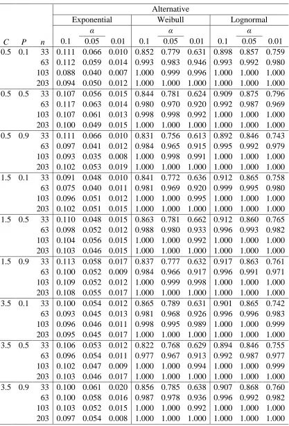
For testing the assumption of exponentiality in AFT models, the U_MOD2 statistic, given by equation (4.4) is used, and is called U_MOD2 _E in this case. The power of this statistic is



 















1/2

1/2 1 2 2

/ 1 ,

i i i i i i i i i i i i

The simulation study is conducted under the following experiment

 There are k = 4 stress levels with values:V₁24,V₂ 26,V₃ 28,andV₄ 30.

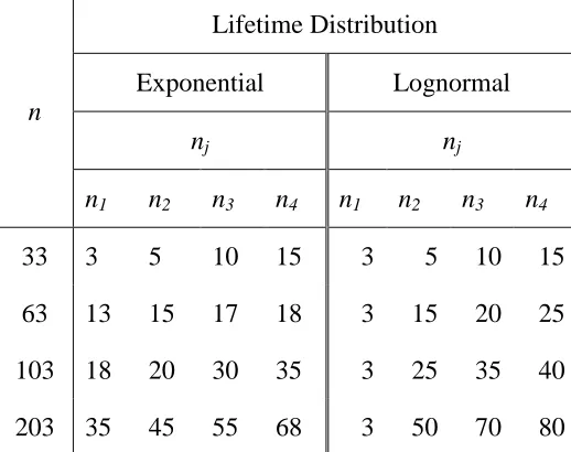
 Different sample sizes, n, and their division on the 4 stress levels, n_j, 1, 2, 3, 4,

j are arbitrary chosen as shown in Table 1.

 Three different initial values of the parameters C and P in equation (4.1) are assumed to be 0.5, 1.5, 3.5 and 0.1, 0.5, 0.9 , respectively. Then, we consider nine different combinations of these values. Three different values of significance levels 0.1, 0.05, 0.01 are considered.

 For each combination of (C, P, n), 1000 samples are generated using Mathcad program from the following distributions

1- Exponential with pdf given by equation (4.3). 2- Weibull with pdf given by

1

( ;_{ij j}, ) ij exp ij , _ij 0, _j, 0,

j j j

t t

f t t

 



   

  

 _{ }

  _   _

 _ _ _ _   

 

  _   _ i1,2,...,nj,

, ,..., 2 ,

1 k

j (5.1)

where t_{i j},i1,2,...,n_j, j1,2,...,k,are the failure times. The shape parameter  is assumed to be independent of the stress levels and is taken to be 0.5. But, the scale parameter _j is assumed to be affected by the stress levels through the inverse power law relationship given by equation (4.1). After substituting (4.1) in (5.1), the pdf will be in the form

1

( ; , , ) exp , 0, , 0.

P P P

j j ij j ij

ij ij

v v t v t

f t C P t C

C C C

 



 

 _{ }

  _   _

 _ _ _ _   

 

  _   _ (5.2)

3- Lognormal with pdf given by equation (4.6), with shape parameter .

5 . 0 / 1  

 For each sample, the MLE of the parameters of these distributions are obtained with tolerance value 0.00001. Then, the U_MOD2 _E statistic is calculated and the power is estimated as:

Power = Number of times rejecting H₀/1000, where

ij

T

H₀: follows exponential distribution with pdf given by equation (4.3). :

1

The estimated power values of U_MOD2 _E statistic in testing the exponential distribution in AFT model are given in Table 2. From this Table, it is seen that the U_MOD2 _E statistic is powerful for testing the exponential distribution versus both the Weibull and lognormal alternatives. This is true whatever the sample size. When the sample size increases, the power of this statistic becomes much better. Sometimes, the power reaches 1. Thus, it could be said that the CPIT method performs well when testing the exponentiality of the AFT model.

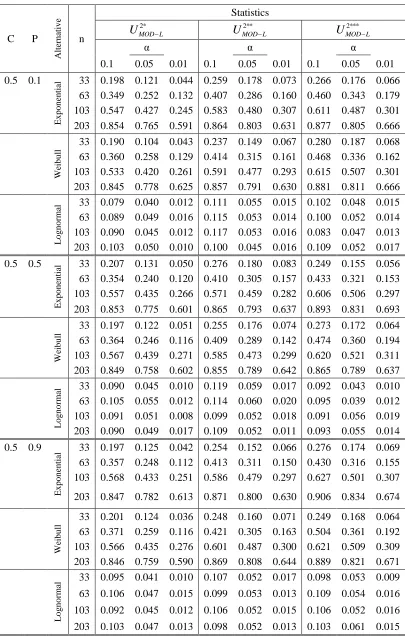
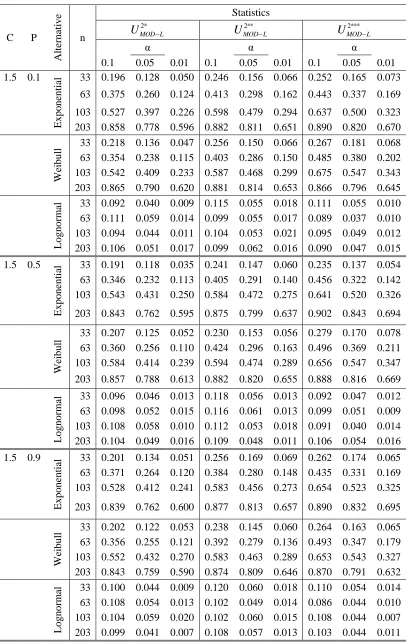
5.2 Testing for the lognormal distribution in AFT model

In this sub-section, we examine the power of the U_MOD2 statistic for testing the assumption of the lognormal distribution in AFT model. The U_MOD2 statistic computed based on the CPIT 1, CPIT 2 and CPIT 3 methods, given by equations (4.7), (4.8), and (4.9) are denoted by U_MOD2* _L, UMOD2** L and

* * * 2

L MOD

U  , respectively.

The simulation study is conducted under the same experiment and procedures as for the exponential distribution, but the values of n_j, j1,..., 4, are different. Since all the log-failure times occurring at the same stress level have the same transformed stress level value x_j, and since CPIT 3 is based on omitting the first 3 observations, then in order to use this transformation, the number of units at the first stress level n₁, should not exceed three test units. This is to avoid the problem of singularity of the matrix (X X_i _i) computed from the matrix X. Thus, the total sample sizes used are redistributed to the 4 stress levels as indicated in Table 1. The distribution of the total sample sizes on the 4 stress levels is arbitrary chosen; taking into consideration that n₁3. In this case it is desired to test the following hypotheses

ij

T

H₀: follows lognormal distribution with pdf given by equation (4.6). :

1

H _NotH0.

The estimated power of U_MOD2* _L, UMOD2** L and

* * * 2

L MOD

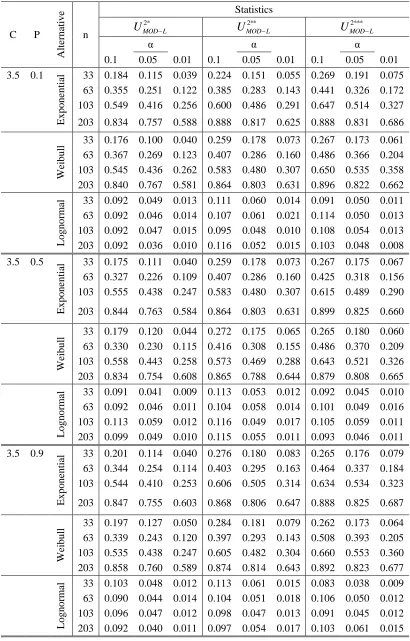
U  statistics in testing the lognormal distribution versus the alternatives, exponential, Weibull and lognormal distributions, are given in Table 3 under different values of C, P, and n. From this Table, it is seen that there are small differences between the power of these statistics. In the majority of cases,

* * * 2

L MOD

6. A Real Life Example

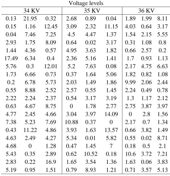
In this Section, we apply the CPIT method to investigate the distribution of times to breakdown of an insulating fluid under three elevated voltage stress. The data used is referred to in Nair (1982). This data represents the times to breakdown of an insulating fluid under three elevated voltage stresses. The data is presented in Table 4 and constitutes the first sixty observations at the three voltage levels.

Nelson (1990) suggested the use of one of the exponential and lognormal distributions to describe the lifetime of insulating fluids. To check the appropriateness of using the lognormal distribution to represent the data given in Table 4, we will use the CPIT statistic, U_MOD2* _L, which does not take into account neither the constancy of the shape parameter of the lognormal distribution nor the inverse power law relationship. First, the log-lifetimes are obtained and then the U_MOD2* _L statistic is applied on these log-failures at each stress level separately. Second, the transformed U values are pooled together from all stress level, and then the U_MOD2* _L statistic is applied on the pooled sample. It is found that, the computed value of U_MOD2* _L statistic, (1.613) exceeds the corresponding critical value (0.187) at significance level 0.05. This indicates that the lognormal distribution is not suitable to represent the lifetime distribution of the times to breakdown data given in Table 4.

To test for the exponential distribution without taking into consideration the inverse power law relationship, the CPIT statistic, U_MOD2 _E is applied on the failure times in the same way as the U_MOD2* _L. The results of using this test indicates that the exponential distribution gives good fit for the data since the computed value of U_MOD2 _E statistic, (0.071) is less than the corresponding critical value (0.187) at significance level

05 . 0



 .

7. Conclusions

that it tests for the underlying distribution regardless the other assumptions of the AFT model.

A simulation study is carried out to explore the power of the CPIT method in validating the underlying distributions in AFT model. First, the CPIT method is used to test for the exponential distribution. Second, three versions of this method are used in testing for the lognormal distribution. It is concluded that the CPIT method is a powerful test in both cases of exponential and lognormal distributions whatever the sample sizes.

Finally, the CPIT method is applied on a real life data that includes the times to breakdown of an insulating fluid to investigate the adequacy of both the lognormal and exponential inverse power law models. The results clarify that the exponential inverse power law model fits the times to breakdown of an insulating fluid better than the lognormal one.

To summarize, the CPIT method is used to assess the GOF of the log-location-scale family of distributions in AFT model. As examples, both the exponential and lognormal lifetime distributions are considered. It is concluded that the CPIT method performs well, so it is recommended to be used in the field of ALT. As a future work, an extension may be made to treat the same problem under different types of censoring.

Table 1: Total sample sizes, n and sub-samples, nj, j=1, ..., 4 in the case of

exponential and lognormal distributions

n

Lifetime Distribution

Exponential Lognormal

nj nj

n1 n2 n3 n4 n1 n2 n3 n4

33 3 5 10 15 3 5 10 15

63 13 15 17 18 3 15 20 25

Table 2: Estimated values of the power for testing the exponential distribution

C P n

Alternative

Exponential Weibull Lognormal

α α α

0.1 0.05 0.01 0.1 0.05 0.01 0.1 0.05 0.01 0.5 0.1 33 0.111 0.066 0.010 0.852 0.779 0.631 0.898 0.857 0.759

Table 3: Estimated values of the power for testing the lognormal distribution

C P

Altern

ati

v

e

n

Statistics 2*

MOD L

U  UMOD L2**  UMOD L2***

α α α

0.1 0.05 0.01 0.1 0.05 0.01 0.1 0.05 0.01

0.5 0.1

Ex

p

o

n

en

ti

al 33 0.198 0.121 0.044 0.259 0.178 0.073 0.266 0.176 0.066

63 0.349 0.252 0.132 0.407 0.286 0.160 0.460 0.343 0.179 103 0.547 0.427 0.245 0.583 0.480 0.307 0.611 0.487 0.301 203 0.854 0.765 0.591 0.864 0.803 0.631 0.877 0.805 0.666

Weib

u

ll

33 0.190 0.104 0.043 0.237 0.149 0.067 0.280 0.187 0.068 63 0.360 0.258 0.129 0.414 0.315 0.161 0.468 0.336 0.162 103 0.533 0.420 0.261 0.591 0.477 0.293 0.615 0.507 0.301 203 0.845 0.778 0.625 0.857 0.791 0.630 0.881 0.811 0.666

Lo

g

n

o

rm

al 33 0.079 0.040 0.012 0.111 0.055 0.015 0.102 0.048 0.015

63 0.089 0.049 0.016 0.115 0.053 0.014 0.100 0.052 0.014 103 0.090 0.045 0.012 0.117 0.053 0.016 0.083 0.047 0.013 203 0.103 0.050 0.010 0.100 0.045 0.016 0.109 0.052 0.017

0.5 0.5

Ex

p

o

n

en

ti

al 33 0.207 0.131 0.050 0.276 0.180 0.083 0.249 0.155 0.056

63 0.354 0.240 0.120 0.410 0.305 0.157 0.433 0.321 0.153 103 0.557 0.435 0.266 0.571 0.459 0.282 0.606 0.506 0.297

203 0.853 0.775 0.601 0.865 0.793 0.637 0.893 0.831 0.693

Weib

u

ll

33 0.197 0.122 0.051 0.255 0.176 0.074 0.273 0.172 0.064 63 0.364 0.246 0.116 0.409 0.289 0.142 0.474 0.360 0.194 103 0.567 0.439 0.271 0.585 0.473 0.299 0.620 0.521 0.311 203 0.849 0.758 0.602 0.855 0.789 0.642 0.865 0.789 0.637

Lo

g

n

o

rm

al 33 0.090 0.045 0.010 0.119 0.059 0.017 0.092 0.043 0.010

63 0.105 0.055 0.012 0.114 0.060 0.020 0.095 0.039 0.012 103 0.091 0.051 0.008 0.099 0.052 0.018 0.091 0.056 0.019 203 0.090 0.049 0.017 0.109 0.052 0.011 0.093 0.055 0.014

0.5 0.9

Ex

p

o

n

en

ti

al 33 0.197 0.125 0.042 0.254 0.152 0.066 0.276 0.174 0.069

63 0.357 0.248 0.112 0.413 0.311 0.150 0.430 0.316 0.155 103 0.568 0.433 0.251 0.586 0.479 0.297 0.627 0.501 0.307

203 0.847 0.782 0.613 0.871 0.800 0.630 0.906 0.834 0.674

Weib

u

ll

33 0.201 0.124 0.036 0.248 0.160 0.071 0.249 0.168 0.064 63 0.371 0.259 0.116 0.421 0.305 0.163 0.504 0.361 0.192 103 0.566 0.435 0.276 0.601 0.487 0.300 0.621 0.509 0.309 203 0.846 0.759 0.590 0.869 0.808 0.644 0.889 0.821 0.671

Lo

g

n

o

rm

al 33 0.095 0.041 0.010 0.107 0.052 0.017 0.098 0.053 0.009

63 0.106 0.047 0.015 0.099 0.053 0.013 0.109 0.054 0.016

103 0.092 0.045 0.012 0.106 0.052 0.015 0.106 0.052 0.016

Table 3: Estimated values of the power for testing the lognormal distribution (Cont.)

C P

A

lt

er

nat

ive

n

Statistics 2*

MOD L

U _ U_{MOD L}2** _ U_{MOD L}2***_

α α α

0.1 0.05 0.01 0.1 0.05 0.01 0.1 0.05 0.01

1.5 0.1

Expo

nent

ial 33 0.196 0.128 0.050 0.246 0.156 0.066 0.252 0.165 0.073

63 0.375 0.260 0.124 0.413 0.298 0.162 0.443 0.337 0.169

103 0.527 0.397 0.226 0.598 0.479 0.294 0.637 0.500 0.323

203 0.858 0.778 0.596 0.882 0.811 0.651 0.890 0.820 0.670

W

ei

bul

l 33 0.218 0.136 0.047 0.256 0.150 0.066 0.267 0.181 0.068

63 0.354 0.238 0.115 0.403 0.286 0.150 0.485 0.380 0.202

103 0.542 0.409 0.233 0.587 0.468 0.299 0.675 0.547 0.343

203 0.865 0.790 0.620 0.881 0.814 0.653 0.866 0.796 0.645

L

ogn

or

m

al 33 0.092 0.040 0.009 0.115 0.055 0.018 0.111 0.055 0.010

63 0.111 0.059 0.014 0.099 0.055 0.017 0.089 0.037 0.010

103 0.094 0.044 0.011 0.104 0.053 0.021 0.095 0.049 0.012

203 0.106 0.051 0.017 0.099 0.062 0.016 0.090 0.047 0.015

1.5 0.5

Expo

nent

ial 33 0.191 0.118 0.035 0.241 0.147 0.060 0.235 0.137 0.054

63 0.346 0.232 0.113 0.405 0.291 0.140 0.456 0.322 0.142

103 0.543 0.431 0.250 0.584 0.472 0.275 0.641 0.520 0.326

203 0.843 0.762 0.595 0.875 0.799 0.637 0.902 0.843 0.694

W

ei

bul

l 33 0.207 0.125 0.052 0.230 0.153 0.056 0.279 0.170 0.078

63 0.360 0.256 0.110 0.424 0.296 0.163 0.496 0.369 0.211

103 0.584 0.414 0.239 0.594 0.474 0.289 0.656 0.547 0.347

203 0.857 0.788 0.613 0.882 0.820 0.655 0.888 0.816 0.669

L

ogn

or

m

al 33 0.096 0.046 0.013 0.118 0.056 0.013 0.092 0.047 0.012

63 0.098 0.052 0.015 0.116 0.061 0.013 0.099 0.051 0.009

103 0.108 0.058 0.010 0.112 0.053 0.018 0.091 0.040 0.014

203 0.104 0.049 0.016 0.109 0.048 0.011 0.106 0.054 0.016

1.5 0.9

Expo

nent

ial 33 0.201 0.134 0.051 0.256 0.169 0.069 0.262 0.174 0.065

63 0.371 0.264 0.120 0.384 0.280 0.148 0.435 0.331 0.169

103 0.528 0.412 0.241 0.583 0.456 0.273 0.654 0.523 0.325

203 0.839 0.762 0.600 0.877 0.813 0.657 0.890 0.832 0.695

W

ei

bul

l 33 0.202 0.122 0.053 0.238 0.145 0.060 0.264 0.163 0.065

63 0.356 0.255 0.121 0.392 0.279 0.136 0.493 0.347 0.179

103 0.552 0.432 0.270 0.583 0.463 0.289 0.653 0.543 0.327

203 0.843 0.759 0.590 0.874 0.809 0.646 0.870 0.791 0.632

L

ogn

or

m

al 33 0.100 0.044 0.009 0.120 0.060 0.018 0.110 0.054 0.014

63 0.108 0.054 0.013 0.102 0.049 0.014 0.086 0.044 0.010

103 0.104 0.059 0.020 0.102 0.060 0.015 0.108 0.044 0.007

Table 3: Estimated values of the power for testing the lognormal distribution (Cont.)

C P

A

lt

er

nat

ive

n

Statistics 2*

MOD L

U _ U_{MOD L}2** _ U_{MOD L}2***_

α α α

0.1 0.05 0.01 0.1 0.05 0.01 0.1 0.05 0.01

3.5 0.1

E

xpo

nent

ial 33 0.184 0.115 0.039 0.224 0.151 0.055 0.269 0.191 0.075

63 0.355 0.251 0.122 0.385 0.283 0.143 0.441 0.326 0.172

103 0.549 0.416 0.256 0.600 0.486 0.291 0.647 0.514 0.327

203 0.834 0.757 0.588 0.888 0.817 0.625 0.888 0.831 0.686

W

ei

bul

l 33 0.176 0.100 0.040 0.259 0.178 0.073 0.267 0.173 0.061

63 0.367 0.269 0.123 0.407 0.286 0.160 0.486 0.366 0.204

103 0.545 0.436 0.262 0.583 0.480 0.307 0.650 0.535 0.358

203 0.840 0.767 0.581 0.864 0.803 0.631 0.896 0.822 0.662

Logn

or

m

al 33 0.092 0.049 0.013 0.111 0.060 0.014 0.091 0.050 0.011

63 0.092 0.046 0.014 0.107 0.061 0.021 0.114 0.050 0.013

103 0.092 0.047 0.015 0.095 0.048 0.010 0.108 0.054 0.013

203 0.092 0.036 0.010 0.116 0.052 0.015 0.103 0.048 0.008

3.5 0.5

E

xpo

nent

ial 33 0.175 0.111 0.040 0.259 0.178 0.073 0.267 0.175 0.067

63 0.327 0.226 0.109 0.407 0.286 0.160 0.425 0.318 0.156

103 0.555 0.438 0.247 0.583 0.480 0.307 0.615 0.489 0.290

203 0.844 0.763 0.584 0.864 0.803 0.631 0.899 0.825 0.660

W

ei

bul

l 33 0.179 0.120 0.044 0.272 0.175 0.065 0.265 0.180 0.060

63 0.330 0.230 0.115 0.416 0.308 0.155 0.486 0.370 0.209

103 0.558 0.443 0.258 0.573 0.469 0.288 0.643 0.521 0.326

203 0.834 0.754 0.608 0.865 0.788 0.644 0.879 0.808 0.665

Logn

or

m

al 33 0.091 0.041 0.009 0.113 0.053 0.012 0.092 0.045 0.010

63 0.092 0.046 0.011 0.104 0.058 0.014 0.101 0.049 0.016

103 0.113 0.059 0.012 0.116 0.049 0.017 0.105 0.059 0.011

203 0.099 0.049 0.010 0.115 0.055 0.011 0.093 0.046 0.011

3.5 0.9

E

xpo

nent

ial 33 0.201 0.114 0.040 0.276 0.180 0.083 0.265 0.176 0.079

63 0.344 0.254 0.114 0.403 0.295 0.163 0.464 0.337 0.184

103 0.544 0.410 0.253 0.606 0.505 0.314 0.634 0.534 0.323

203 0.847 0.755 0.603 0.868 0.806 0.647 0.888 0.825 0.687

W

ei

bul

l 33 0.197 0.127 0.050 0.284 0.181 0.079 0.262 0.173 0.064

63 0.339 0.243 0.120 0.397 0.293 0.143 0.508 0.393 0.205

103 0.535 0.438 0.247 0.605 0.482 0.304 0.660 0.553 0.360

203 0.858 0.760 0.589 0.874 0.814 0.643 0.892 0.823 0.677

Logn

or

m

al 33 0.103 0.048 0.012 0.113 0.061 0.015 0.083 0.038 0.009

63 0.090 0.044 0.014 0.104 0.051 0.018 0.106 0.050 0.012

103 0.096 0.047 0.012 0.098 0.047 0.013 0.091 0.045 0.012

Table 4: Observed times to breakdown in minutes of an insulating fluid*

Voltage levels

34 KV 35 KV 36 KV

0.13 21.95 0.32 2.68 0.89 0.04 1.89 1.99 8.11 0.15 1.16 12.45 3.09 2.32 11.15 4.03 0.64 3.17 0.04 7.46 7.25 4.5 4.47 1.37 1.54 2.15 5.55 2.93 1.75 8.09 0.64 0.02 3.17 0.31 1.08 0.8 1.44 4.36 0.57 4.95 3.63 1.82 0.66 2.57 0.2 17.49 6.34 0.4 2.36 5.16 1.41 1.7 0.93 1.13

5.76 0.3 12.01 5.2 7.63 0.08 2.17 4.75 6.63 1.73 6.66 0.73 0.37 1.64 5.06 1.82 0.82 1.08 0.2 6.78 5.73 2.03 1.49 1.86 9.99 2.06 2.44 0.55 8.88 2.52 2.57 0.55 1.45 2.24 0.49 0.78 2.22 2.24 2.37 0.54 3.17 3.19 1.3 1.17 2.12 0.63 4.67 8.75 0 1.78 2.77 2.75 3.87 3.97 4.77 2.45 4.66 3.04 3.97 14.09 0 2.8 1.56 7.38 5.23 7.69 10.88 0.37 0 2.17 0.7 1.34 0.43 11.22 4.86 3.93 1.63 13.57 0.66 3.82 1.49 4.63 2.49 4.27 5.34 0.01 5.82 0.55 0.02 8.71 4.68 0 1.28 0.47 1.45 7 0.18 0.5 2.1 5.43 0.35 2.89 0.62 10.52 0.18 10.6 3.72 7.21 2.83 0.22 16.9 1.65 3.54 1.36 1.63 0.06 3.83 5.19 0.95 1.51 0.79 8.93 1.21 0.71 3.57 5.13

* Source: Nair (1982).

References

1. Bagadonavičius, V., Cheminade, O. and Nikulin, M. (2004). Statistical planning and inference in accelerated life testing using the CHSS model. Journal of Statistical Planning and Inference, 126, 535-551.

2. Bagadonavičius, V., Kruopis, J. and Nikulin, M. (2011). Nonparametric Tests for Censored Data. ISTE and J. Wiley, London.

3. Bagadonavičius, V., Levuliene, R.T. and Nikulin, M. (2013). Chi-squared goodness-of-fit tests for parametric accelerated failure time models. Communications in Statistics - Theory and Methods, 42, 2768-2785.

4. Bagadonavičius, V. and Nikulin, M. (2002). Accelerated Life Models: Modeling and Statistical Analysis. Champman and Hall/CRC, Boca Raton.

5. Balakrishnan, N., Chimitova, E., Galanova, N. and Vedernikova, M. (2013). Testing goodness of fit of parametric AFT and PH models with residuals. Communications in Statistics – Simulation and Computation, 42, 1352-1367. 6. D'Agostino, R. and Stephens, M. (1986). Goodness-of-Fit Techniques. Marcel

7. Eguchi, S. (1992). The projection method for accelerated life test model in bivariate Exponential Distributions. Hiroshima Math., 22, 185-193.

8. Galanova, N. S., Lemeshko, B. Y. and Chimitova, E. V. (2012). Using nonparametric goodness-of-fit tests to validate accelerated failure time. Optoelectronics, Instrumentation and Data Processing, 48, 580-592.

9. Lawless, J. F. (2003). Statistical Models and Methods for Lifetime Data. John Willey and Sons, New York, NY.

10. Nair, V. N. (1982). Q-Q Plots with confidence bands for comparing several populations. Scandinavian Journal of Statistics, 9, 193-200.

11. Nelson, W. B. (1990). Accelerated Testing: Statistical Models, Test Plans, and Data Analysis. John Wiley and Sons, New York, NY.

12. O'Reilly, F. J. and Quesenberry, C. P. (1973). The conditional probability integral transformation and applications to obtain composite chi-square goodness of fit tests. The Annals of Statistics, 1, 74-83.

13. O'Reilly, F. J. and Stephens, M. A. (1982). Characterizations and goodness of fit tests. Journal of the Royal Statistical Society, 44, 353-360.

14. Quesenberry, C. P., Giesbrecht, F. G. and Burns, J. C. (1983). Some methods for studying the validity of normal model assumptions for multiple samples. Biometrics, 39, 735-739.

15. Sethurman, J. and Singpurwalla, N. D. (1982). Testing of hypothesis for distributions in accelerated life testing. Journal of American Statistical Association, 77, 204-208.

16. Teng, S. L. and Yeon, K. P. (2002). A least-squares approach to analyzing life-stress relationship in step-life-stress accelerated life tests. IEEE Transactions on Reliability, 51, 177-182.