SYSTEMATIC REVIEW
Ravenous wolves revisited: a systematic
review of offending concentration
Natalie N. Martinez
1, YongJei Lee
2, John E. Eck
1*and SooHyun O
1Abstract
Background: Numerous studies have established that crime is highly concentrated among a small group of offend-ers. These findings have guided the development of various crime prevention strategies. The underlying theme of these strategies is that by focusing on the few offenders who are responsible for most of the crime, we can prevent the greatest amount of crime with the fewest resources. Nevertheless, there has been no systematic review of the many studies, so it is possible that the accepted understanding among researchers and practitioners is based on a few prominent studies that are misleading. Further, we do not know how concentrated crime is among offenders, given the variety of ways researchers report their findings. This paper systematically reviews this literature and uses meta-analysis to determine how confident we can be that crime is concentrated among a few offenders.
Methods: We first systematically reviewed the literature and found 73 studies on the concentration of crime among offenders. From those studies, we identified 15 studies on the prevalence of offending and 27 studies on the fre-quency of offending that provided data suitable for analysis. We then performed a meta-analysis of those studies to examine how crime is concentrated among the worst offenders and how that concentration varies between different types of offenders.
Results: We found that crime is highly concentrated in the population and across different types of offenders. Little variation in concentration exists between youths and adults or between American offenders and those from other countries. We found more variation between males and females in the concentration of offending, though we believe this may be due to the more limited data on female offenders.
Conclusions: The systematic review and meta-analysis we present here is the first study of its kind on offending con-centration. This is an important step in closing this gap in the crime prevention literature, but we encourage making updates to this systematic review as new literature becomes available, and using alternate methods of summarizing these studies that could challenge these findings.
Keywords: Crime concentration, Offending, Systematic review, Meta-analysis
© The Author(s) 2017. This article is distributed under the terms of the Creative Commons Attribution 4.0 International License (http://creativecommons.org/licenses/by/4.0/), which permits unrestricted use, distribution, and reproduction in any medium, provided you give appropriate credit to the original author(s) and the source, provide a link to the Creative Commons license, and indicate if changes were made.
Background
If crimes were equally distributed in society, then 10% of all offenders would account for 10% of all crimes, 20% of offenders would account for 20% of all crimes, and so on. Decades of research on offenders has shown that this is not the case. In fact, those studies have repeatedly found that the distribution of offending is skewed and that crime is highly concentrated among a small proportion
of offenders (e.g., Elonheimo et al. 2014; Glueck and Glueck 1950; Harer 1995; Piquero and Buka 2002; Shan-non et al. 1988; Wolfgang et al. 1972). For example, Wolf-gang et al. (1972) found that 6% of the males in the 1945 Philadelphia birth cohort accounted for about 52% of all the police contacts; Sampson and Laub (2003) found that less than 3% of the Boston males in their sample were responsible for 51% of arrests after age 31; Harer (1995) found that about 6% of federal parolees accounted for 39% of all rearrests; and Ambihapathy (1983) found that about 8% of female offenders in Ottawa, Ontario accounted for about 36% of the arrests among that
Open Access
*Correspondence: john.eck@uc.edu
1 School of Criminal Justice, University of Cincinnati, Cincinnati, OH 45221, USA
group. As these examples illustrate, studies that provide concentration statistics do not necessarily report them using the same benchmarks (e.g., 5, 10, or 20% of offend-ers), and it appears that the concentration of crime can vary between studies due to differences in their samples’ characteristics.
So then, just how concentrated is offending? The answer to our question may become clearer if we turn our attention to cumulative distributions of offending. Cumulative distributions provide a count of the crimes committed by each of the individuals in a cohort (or sam-ple), who can then be ranked in declining order of the number of crimes they have committed. When graph-ing this distribution, the horizontal (x) axis is measured in percentages, so the leftmost value represents the most crime-involved percentage of individuals (e.g. the “worst” 1%) and the rightmost value represents 100% of the group being studied. The points on the vertical (y) axis repre-sent the percentage of all crimes committed by a given percentage of offenders along the x axis. A graph of the distribution of offending concentration would resemble a reclining letter “J,” with the tallest bars at the leftmost portion of the graph that gradually flatten out when mov-ing toward the right (see Eck et al. 2007).
Spelman (1986) compared J-curves he constructed from the cumulative distributions of offending from four studies (two Philadelphia cohorts plus London and Racine cohorts). Although these studies differed in their locations, years, and methods, Spelman (1986) found that the curves from the different studies were very similar in shape. Across the four studies, the 10% of offenders most involved in crime accounted for about 40% of all offenses.
Criminologists and practitioners have long relied on the principle of crime concentration to guide crime prevention strategies. Through selective incapacita-tion, for example, the offenders responsible for the most crimes receive the longest sentences while other offend-ers receive shorter ones. By focusing resources on those offenders who contribute the most to the crime prob-lem, selective incapacitation can be an effective strategy for preventing future crime as well as minimizing prison operating costs (Auerhahn 1999; Greenwood and Abra-hamse 1982). Another example comes from the princi-ples of effective rehabilitation, which hold that treatment is most effective at preventing crime when its intensity matches the offender’s recidivism risk level (Gendreau 1996), and offenders at the greatest risk of recidivat-ing benefit most from intense rehabilitation programs (Lowenkamp and Latessa 2004). Finally, situational crime prevention efforts are aimed at changing offenders’ per-ceptions about the risks and rewards of crime opportu-nities (Clarke 1997). If a few offenders are responsible for most of the crime, then blocking opportunities can
greatly reduce crime by changing these offenders’ per-ceptions about its benefits.
Despite the large number of studies published on offenders and the importance of repeat offending to crime prevention, researchers have not synthesized this research. The lack of a systematic review creates two potential problems. First, our understanding of crime concentration among offenders maybe biased by the find-ings of a few prominent studies, because we may have ignored contradictory findings from lesser known stud-ies. Even if our understanding of offending concentration is reasonably correct, we neither know how much this concentration varies across different groups, nor can we estimate the average concentration. The purpose of this paper is to close these gaps in the literature. We aim to gain insight on how concentrated crime is when we con-sider all the studies on this topic, how much variation exists in crime concentration among the worst offenders, and how crime concentration compares across the differ-ent groups that differdiffer-ent researchers have studied.
The literature on offending concentration
Evidence of crime concentration among offenders dates back many decades. For example, Shaw and McKay (1942) mapped the home addresses of boys arrested in Chicago. Only one quarter of Chicago’s boys lived in the areas of the city with the highest juvenile arrest rates yet boys from these areas accounted for 50–60% of all the boys arrested during the years they studied. Shaw and McKay (1942) focused on the number of offenders arrested rather than the number of arrests per offender, but their results nevertheless demonstrate that offending is not equally distributed.
Scholarly interest in quantifying offending behavior continued with Glueck and Glueck’s research on delin-quent boys in Boston. The boys in Glueck and Glueck’s (1950) sample received between one and ten court con-victions, and they counted the number of boys convicted in court once, twice, and so on for all 500 offenders. This publication provides an early example of the crime con-centration statistics needed to create a cumulative distri-bution of offending. Unfortunately, their critics labeled the Gluecks’ body of research atheoretical because it focused on individual criminogenic traits as causes of criminality, which contrasted with the criminology field’s emphasis on social causes of crime at the time (Cullen 2011). Though forced into the criminological shadows for many years, the Gluecks’ work nevertheless laid the groundwork for the later criminal career research that brought attention to the concentration of offending.
and frequency. Prevalence of offending refers to the pro-portion of people in a population who engage in crime or delinquency (Farrington 2015; Rocque et al. 2015b; Till-man 1987) while frequency refers to the number of times an individual offends (Farrington 2015; Tillman 1987). Thus, prevalence statistics describe groups that comprise both non-offenders and offenders whereas frequency sta-tistics describe only the behavior of offenders. In 1972, Wolfgang and his colleagues published Delinquency in a Birth Cohort, a landmark study on offending. Wolfgang et al. (1972) analyzed the juvenile police contact data for a birth cohort that included all boys born in Philadelphia in 1945 and still residing there 10 years later. As mentioned earlier, Wolfgang et al. (1972) found that a small number of high-frequency offenders in the cohort were respon-sible for about half of all the police contacts. Referred to in the study as “chronic” offenders, this small number of boys represented 6% of the entire cohort (an indicator of the prevalence of offending among all boys in the cohort) and 18% of the offenders in the cohort (and indicator of the frequency of offending among delinquents). The sta-tistics on chronic offenders are the stasta-tistics most often cited from their study, but Wolfgang et al. (1972) pro-vided statistics on the full distribution of offending in the cohort as well.
Wolfgang et al.’s (1972) identification of a small group of high-frequency offenders renewed interest in crimi-nal career research. Similar studies conducted on birth cohorts in Wisconsin (Shannon et al. 1988), Denmark (Van Dusen and Mednick 1984), Puerto Rico (Nevares et al. 1990), and Sweden (Wikström 1990), for example, have been published over the years. Birth cohort studies are ideal because they represent a population of individu-als, but prevalence and frequency statistics do exist for samples of individuals as well (e.g., Brame et al. 2004; Liu et al. 1997; Piquero and Buka 2002; Piquero et al. 2007).
Offending concentration studies differ widely in the types of people they study, the measures of crime they use, and the terminology they use to describe offend-ing concentration. Some studies have focused only on males (e.g., Glueck and Glueck 1950; Tracy et al. 1990; Van Dusen and Mednick 1984; Wolfgang et al. 1972), only on females (e.g., Warren and Rosenbaum 1986) or both (e.g., Hamparian et al. 1978; Harer 1995; Nevares et al. 1990; Shannon et al. 1988). Likewise, many studies have focused exclusively on juveniles (e.g., Nevares et al. 1990; Wolfgang et al. 1972), and to a lesser extent only on adults (e.g., Sampson and Laub 2003). The measures of crime used in offending concentration studies usually range from arrests (e.g., Ambihapathy 1983; Brame et al. 2004; Fry 1985; Tillman 1987) and contacts with police (e.g., Nevares et al. 1990; Van Dusen and Mednick 1984; Wolfgang et al. 1972) to charges (e.g., Collins and Wilson
1990) and convictions (e.g., Carrington et al. 2005; Far-rington and Maughan 1999; Piquero et al. 2007), but also include combining all offending into one generic “offense” measure (e.g., Cernkovich et al. 1985; Far-rington et al. 2003; Piquero and Buka 2002). However, a few studies have used other measures of crime, like the number of court sentences and legal punishments (Liu et al. 1997), jail bookings (Yunker et al. 2001), and police investigations (Piquero et al. 2008).
The way researchers define the worst offenders varies from study to study. Wolfgang et al. (1972) referred to them as chronic offenders, which they defined as any boy responsible for at least five police contacts. Several stud-ies have followed Wolfgang et al.’s (1972) example and defined chronic offenders in their samples as individuals responsible for at least five offenses (e.g., Ambihapathy 1983; Carrington et al. 2005; Collins 1987; DeLisi and Scherer 2006; Liu et al. 1997; Piquero and Buka 2002; Piper 1983; Piquero et al. 2008; Shannon et al. 1988; Van Dusen and Mednick 1984). However, this definition of the worst offenders is not the same in all studies. Some studies have referred to offenders as chronic if they were responsible for at least three offenses (e.g., Mednick et al. 1984; Nevares et al. 1990; Tillman 1987), at least four offenses (e.g., Schumacher and Kurz 2000), at least nine offenses (e.g., Farrington and Maughan 1999), at least 15 offenses (e.g., Skrzypiec et al. 2005), or a mixed number of offenses (e.g., Sampson and Laub 2003;1 Yunker et al. 2001)2. Still others make no such distinction between offenders in terms of their frequency (e.g., Beaver 2013; Beck and Shipley 1987; Brame et al. 2004; Collins and Wilson 1990; Elonheimo et al. 2014; Glueck and Glueck 1950; Harer 1995; Piquero et al. 2007; Warren and Rosen-baum 1986). As these examples illustrate, the concept of chronic offending is arbitrarily defined in the literature. In this study, we focus not on offenders who have com-mitted a minimum number of crimes, but rather on the worst offenders in the distribution. We define the worst offenders as those with the highest frequency of offend-ing, and we divide them into deciles to describe the varia-tion in the concentravaria-tion of crime among them (we discuss this more in “Analysis” section).
Environmental criminology and offending concentration Offenders are the central focus of traditional criminology, which attempts to explain involvement and desistance from crime through differences in offenders’ cognitive,
1 Sampson and Laub (2003) defined chronic offenders as the 10 percent
highest frequency offenders.
2 In Yunker et al.’s (2001) report, chronic offenders included individuals
social, and moral development (Lilly et al. 2015). In contrast, environmental criminology focuses on crime events and the factors that create opportunities for those events to occur (Clarke 2004; Wilcox et al. 2012). While traditional criminology focuses exclusively on offenders, environmental criminology acknowledges that victims, guardians, and other third-party actors play an impor-tant role in facilitating or blocking opportunities for crime, and many crime prevention strategies focus on the actions of these other actors (Scott 2005). Nevertheless, offenders are still critically important in environmen-tal criminology because it is the offender’s perceptions of opportunity that matters (Clarke 1997). Even though others may influence their decisions, it is the offender who ultimately chooses to commit crime. Consequently, the concentration of crime among offenders should be of equal importance to environmental criminology as the concentration of crime among places and victims. In particular, if crime is highly concentrated among rela-tively few offenders, then this implies that few individu-als recognize that suitable crime opportunities exist. It also implies that successful situational crime prevention efforts must disproportionately affect these high-fre-quency offenders.
Purpose of the study
Spelman and Eck (1989) emphasized the value of under-standing crime concentration for developing effective crime prevention. Recognizing that crime is highly con-centrated among a small number of “ravenous wolves” (Eck 2001; Spelman and Eck 1989) can help to reduce crime by guiding strategies that remove opportuni-ties for offending among this group. However, we know of no other publications since Spelman (1986) and later Spelman and Eck (1989) that have analyzed the cumula-tive distribution of offending across multiple studies.
After more than 25 years, we believe these efforts need an update. Our purpose in undertaking this task is to synthesize what we know from past studies about the concentration of offending, examine how crime concen-tration varies among the worst offenders, and compare the concentration of crime across the different offender groups that have been studied over the years. To accom-plish this, we first conducted a systematic review of the literature on repeat offending and then meta-analyzed the studies we collected. In the next section, we describe how we identified and analyzed the literature on this topic.
Methods
Criteria for inclusion and exclusion
Each study we located for our systematic review had to meet three criteria before we would include it in our
analysis. First, the study had to be written in English. Sec-ond, the study had to contain original empirical data describing the distribution of crime over possible offend-ers (as opposed to a secondary report of other scholars’ findings). Third, the study had to provide data that allowed us to determine the percentage of offenders in its sample and percentage of crimes associated with those offenders.3
Data sources and search strategy
We4 conducted a systematic review of the literature on offending concentration. To find studies, we began by reviewing articles that summarized past research on repeat offending. A major theme across these publica-tions was the distinction they gave to Wolfgang et al. (1972) as the seminal study on the concentration of offending within a population (DeLisi and Piquero 2011; Edelstein 2016; Farrington 1992; Petersilia 1980; Spelman 1986). Following the logic that subsequent studies on offending concentration would have also referenced this work, we performed a Google Scholar citation search for Delinquency in a Birth Cohort and limited our findings to works published in English. Although that search pro-duced 1870 results, Google Scholar’s algorithm limits the reviewable results to 1000 for any given search (Beel and Gipp 2009). We reviewed the titles and abstracts for these 1000 results and located 50 relevant studies for our analysis.
We recognize the possibility that some relevant studies on offending concentration may not have cited Wolfgang et al. (1972). Moreover, a search for only studies citing Wolfgang et al. (1972) would necessarily exclude any rel-evant studies published before it. Therefore, we located additional studies through manual searches of the litera-ture reviews from the studies already included in our analysis. We also solicited fellow scholars who attended preliminary presentations of our analysis to recommend studies. Throughout this process, we noted frequently used keywords in relevant studies including: offender/ offending concentration, chronic offender/offending, repeat offender/offending, offender/offending prevalence, habit-ual offender/offending, persistent offender/offending, and recidivist/recidivism. We used the keywords to create automated search notifications of two ProQuest and
3 The studies had to provide percentages or at least raw counts of offenders
and their crimes that we could use to calculate percentages.
4 The pronoun “we” is used for simplicity. The lead author was
three EBSCO databases available through the University of Cincinnati Libraries to find additional studies our other search methods may have missed.5 We used an iterative process to search the databases, meaning that we repeated our searches as we identified additional rele-vant keywords. Many results overlapped between our various search methods, but we identified an additional 23 studies through the literature review and database searches that we did not find in the Google Scholar search.
Coding protocol
As we noted earlier, the studies eligible for inclusion had to provide data that allowed us to determine the percent-age of offenders and crime. For each study’s data, we con-structed sets of x–y ordered pairs representing a given percentage of people (x) and their associated percent-age of crime (y). For example, Wolfgang et al. (1972) cal-culated that 6% of boys accounted for 51.8% of all police contacts, so the ordered pair for this data point is (6, 51.8). We coded each data point according to whether it repre-sented a measure of offending within a group of offend-ers and non-offendoffend-ers, or whether it only measured the frequency of offending within a group of offenders. For example, in Wolfgang et al. (1972), the 6% of the popula-tion of boys that accounted for 51.8% of police contacts also represented 18% of all offenders. The x–y ordered pairs (6, 51.8) and (18, 51.8) represent measures of offend-ing prevalence and frequency for these data, respectively. For simplicity, throughout this paper we refer to distribu-tions of the former as “prevalence” and distribudistribu-tions of the latter as “frequency.” We also coded each data point according to the study’s decade of publication, offenders’ gender (i.e., male or female), age (i.e., youth or adult) and location (i.e., United States or other country).
In total, we found 73 studies that provided 621 data points on offending concentration.6 However, we restricted our analysis to only those studies that provided complete crime distributions (see the next section for an explanation). Table 1 summarizes the characteristics of the studies included in our analysis. Males, youths, and people in the United States were the most common sub-jects of research in these studies compared to females, adults and people outside the United States.
5 The ProQuest databases included Criminal Justice and Dissertations and
Theses. The EBSCO databases included Academic Search Complete, Crimi-nal Justice Abstracts, ERIC, and SocINDEX.
6 We did not code studies that provided duplicate data points. For
exam-ple, Piper (1983, 1985) provided some of the same concentration statistics on offending in the 1958 Philadelphia birth cohort. Similarly, Guttridge et al. (1983) provided some of the same statistics representing the distribution of violent offending across Danish males as Van Dusen and Mednick (1984). We coded only Piper’s (1983) and Van Dusen and Mednick’s (1984) findings for analysis because they provided a greater number of relevant statistics.
Analysis
Because this is the first meta-analysis of offending con-centration, we had no guide to follow for combining the results from multiple studies. We used the visual binning tool in SPSS 21 to sort our unweighted data points7 into groups, or bins, along the x-axis. We created 100 bins that ranged in value from 1 to 100% of offenders. We assigned data points to bins according to their x-axis value8 and calculated the median y-axis value for each bin.9 We then calculated a logarithmic curve to represent the cumulative distribution of offenders and crime (see Lee et al. 2017). Using only logarithmic curves in our analysis standardizes our comparisons of offender groups and allows us to compare crime concentration across offenders, victims, and places (see Eck et al. 2017, this issue).
Of the 73 studies we collected for the systematic review, 30 provided complete crime distributions, and 43 provided only partial distributions. Complete crime distributions were those that included at least two data points between, but not including, zero and 100%. “Par-tial” crime distributions were those that included only one data point. We chose to restrict our analysis to only those studies that provided “complete” prevalence or frequency distributions of crime. We chose to do this because a single data point may not adequately repre-sent a study’s distribution, and we wanted to reduce the chance of our results being unduly influenced by studies reporting single data points. To test whether excluding partial data distributions changed the results of our anal-ysis, we created prevalence and frequency distributions using all our data (including partial distributions) and then compared those distributions to their correspond-ing complete distributions (which did not include partial distributions). Figure 1 shows that there is little difference overall between the complete and partial distributions for either the prevalence or frequency of offending, as judged by the fit of a logarithmic curve to the distributions.
Researchers often compare offenders on their demo-graphics (e.g., age, gender, and race), location (e.g., cross-national comparisons), types of offenses commit-ted (e.g., property crime and violent crime), and crime data sources (e.g., official records and self-reports).
7 We tested whether weighting our data would change our results. We
weighted the y value of each data point by its respective study sample size (w) and then calculated the weighted median (wyi) for each bin (i) as a measure of weighted central tendency. We found no substantial difference between the logarithmic curves for the weighted and unweighted data (see Appendix A). We chose to use unweighted data to simplify the interpreta-tions of our results.
8 The Wolfgang et al. (1972) statistic referenced above is in the sixth bin
along the x-axis, which represents 6% of offenders.
9 We chose to use the median to account for (1) variation in y values at
Making such comparisons across studies requires that (1) offender and offense characteristics are measured the same way and that (2) a sufficient number of studies exist with data on those measures. The studies we collected contained many of these characteristics on offenders,
but our conservative decision to focus only on com-plete crime distributions limited the types of compari-sons available in our data. For example, comparicompari-sons of data from official records and self-reports suggest that offending prevalence and frequency differs across these Table 1 Characteristics of studies in the meta-analysis
a Non-US prevalence data included studies from: England (2), Denmark (1), Finland (1) and Puerto Rico (1)
b Non-US frequency data included studies from: Australia (2), Canada (2), England (2), China (1), Denmark (1), Europe (1), and Puerto Rico (1)
Characteristics Prevalence Frequency
Number of studies Number of ordered pairs Number of studies Number of ordered pairs Number of studies included in both
Publication decade
1950–1959 0 0 1 10 0
1960–1969 0 0 0 0 0
1970–1979 1 3 2 8 1
1980–1989 3 26 9 105 3
1990–1999 4 43 6 74 4
2000–2009 6 80 8 88 4
2010–2014 1 2 1 3 0
Type of offender
Adult 3 34 7 71 2
Youth 7 64 12 110 6
Male 13 108 14 119 11
Female 5 17 7 35 4
United States 10 95 17 170 8
Non-United Statesa, b 5 59 10 118 4
Studies analyzed 15 154 27 288
(Studies identified) (55) (263) (44) (358)
two types of data sources (Babinski et al. 2001; Kirk 2006). Some of the studies we collected for the system-atic review included self-report or official records data, but limiting our analysis to complete crime distributions excluded the self-report data on offending prevalence.
In addition to an overall analysis of the prevalence and frequency of offending across the various studies that met our inclusion criteria, we present three other comparisons. We compare the offending distributions between males and females, youths and adults, and the United States and other countries. We chose these three because we had sufficient data for these comparisons. We would have liked to make other comparisons, but we were limited by the original study authors’ data collec-tion methods and the fact that there is no standard pro-cedure for defining characteristics and collecting data on offenders.
Results
We chose to display crime concentration by graphing the logarithmic curves created using the x–y ordered pairs for our data points. Visually, a straight diagonal line from the graph’s origin to the ordered pair representing 100% of the people and 100% of crime would indicate no concentration. Offending would be evenly spread across the people studied. Conversely, a curve with all percent-ages of crime (on the y-axis) greater than the cumulative percentage of offenders (on the x-axis) shows concentra-tion. The more the curve bows toward the upper left of the graph, the greater the crime concentration. Substan-tively, crime concentration is greater when fewer offend-ers account for a large proportion of crime.
Overall offending prevalence and frequency
We began our analysis by comparing the cumulative distributions of offending prevalence and frequency across all our studies. We calculated the prevalence and frequency curves using 154 data points from 15 stud-ies and 288 data points from 27 studstud-ies, respectively. In Fig. 2, the solid line represents the prevalence curve and the dashed line represents the frequency curve. The prevalence curve represents the distribution of offending across a “population” containing both offenders and non-offenders. In contrast, the frequency curve reflects the crime concentration only among individuals who have committed at least one offense (i.e., offenders). The prev-alence distribution shows more crime concentration than the frequency distribution. This is expected given that offending is a rare occurrence (i.e., most people in the population do not commit crime). For example, the 10% of the most criminally-active people account for around 66% of crime, whereas the most active 10% of offenders account for around 41% of crime (see Fig. 2).
Youths and adults
Research has shown that involvement in offending differs between youths10 and adults. The prevalence of offending tends to reach its peak in late adolescence and then declines rapidly by early adulthood.11 This pattern is commonly referred to as the “age-crime curve” (Far-rington 1986; Hirschi and Gottfredson 1983; Piquero et al. 2003). Hirschi and Gottfredson (1983) contend that the age-crime curve is invariant, meaning that the pat-tern of involvement is the same for all types of offenders. If the prevalence of offending follows a stable pattern that predicts a sharp decline in early adulthood, then there would be no need to examine changes in offending over the life course through criminal career research (Rocque et al. 2015a). Although youths are more likely than adults to be involved in crime, it is unclear whether the preva-lence of offending differs within each group.
It is also unclear whether youths and adults differ in the frequency of their offending. Hirschi and Got-tfredson (1983) claim that the frequency of offend-ing follows the same pattern as prevalence. In other words, the sharp decline in the age-crime curve that occurs in early adulthood reflects both a decrease in
10 Offenders were labeled as youths or adults based on the original studies’
categorizations. Youth and adult offenders were defined differently across studies. For example, Beck and Shipley (1987) studied adult offenders age 17 and older whereas Wolfgang et al. (1972) studied youth offenders age 17 and younger.
11 Graphically, a histogram of offenders arranged in age from youngest to
oldest along the horizontal axis would show a gradual increase in the preva-lence of offending from childhood to late adolescence, and then a sharp decrease in prevalence among adults (see Hirschi and Gottfredson 1983).
the prevalence of offending and a decrease in the fre-quency of offending (Piquero et al. 2003). However, the research on offending generally does not support this view (for a review, see Piquero et al. 2003). In contrast, Blumstein et al. (1988) argue that while the decline could be the result of a large proportion of offenders desisting from crime as young adults, this does not mean that those who continue to offend necessarily do so less frequently.
To examine these potential differences in offending prevalence and frequency, we used a combination of data points from studies of (1) only youths (2) only adults, and (3) both youths and adults. In the third category, we retained the data points from studies that differenti-ated between crimes committed by youth offenders and crimes committed by adult offenders. We estimated the prevalence curves using 64 data points from 7 studies for youths and 34 data points from 3 studies for adults. We calculated the frequency curves using 110 data points from 12 studies for youths and 71 data points from 7 studies for adults.
In Figs. 3 and 4, the dashed lines represent the youth curves and the solid lines represents the adult curves. The prevalence curves in Fig. 3 show little difference in the concentration of offending among youths and adults in the population. It appears that the worst (i.e., the most criminally active) 10% of youths account for a slightly smaller proportion of their age group’s crime (about 37%) than the most active 10% of adults (about 41%). In Fig. 4, we found more concentration in the frequency of offend-ing among the adult offenders than among the youth offenders. However, the standard errors of each curve indicate that the graphs are not substantially different
from each other in terms of offending concentration (see Appendix B). Our results suggest that the prevalence and frequency of offending is similar between youths and adults.
Males and females
Males and females differ in both the prevalence and fre-quency of offending. Males are more likely to offend, and those who do offend tend to commit crime with greater frequency than female offenders (D’Unger et al. 2002). This would suggest that the prevalence of offending is less concentrated among the male population and that the frequency of offending is more concentrated among male offenders. To compare male and female offending, we used a combination of data points from studies of (1) only males (2) only females, and (3) both males and females. In the last category, we retained the data points from studies that differentiated acts committed by males from those committed by females. We calculated the prevalence curves using 108 data points from 13 studies for males and 17 data points from 5 studies for females. We calculated the frequency curves using 119 data points from 14 studies for males and 35 data points from 7 stud-ies for females.
In Figs. 5 and 6, the solid lines represent the male curves and dashed lines represent the female curves. The comparison of the prevalence curves in Fig. 5 shows some difference in the prevalence of offending among males and females in their respective populations. According to our results, the prevalence of offending is somewhat more concentrated among males. This finding contra-dicts our expectations, as it implies that offending is more Fig. 3 Adult and youth offending prevalence
y = 21.203ln(x) - 7.6123 R² = 0.9334
y = 24.342ln(x) - 22.824 R² = 0.8664
0 10 20 30 40 50 60 70 80 90 100
0 10 20 30 40 50 60 70 80 90 100
Cu
mu
la
v
e
pe
rc
en
ta
ge
of
cr
im
e
Cumulave percentage of offenders (Frequency) Adult
Youth
widespread among females than among males. However, these differences are small for the males and females who are the most involved in crime. For example, the most crime-involved 10% of males account for around 66% of the crime whereas the same 10% of females account for 59% of crime. In the frequency curve comparison, we again find some difference between males and females. The frequency of offending is more concentrated among male offenders and the males who repeatedly offend are
responsible for a slightly greater proportion of crime than are their female counterparts. Using the 10% of indi-viduals who are the most involved in crime as a bench-mark, this percentage of males and females account for around 42 and 37% of crime, respectively. However, given the notable disparity in numbers of studies on male and female offending, these findings must be treated with some caution, as we will discuss later in the paper.
The United States and other countries
Comparing the distributions of offending between the United States and other countries allows us to examine crime concentration across different social, cultural, and legal contexts (Farrington 2015; Farrington and Wik-strom 1994). Using Wolfgang et al.’s (1972) definition of chronic offenders, Rocque et al. (2015b) examined the prevalence of chronic offenders in an international sample and found that they were more common in the United States and European countries than in Latin American countries. They created a proxy for the differ-ent cultural contexts by grouping the countries into five clusters based on similarities in their social welfare states. Clustering the United States with Ireland, Rocque and his colleagues found that chronic offenders comprised 10.9% of that sample, compared to 9.4% (“Western Europe”), 7.8% (“Northern Europe”), 6.2% (“Mediterranean Europe”), 5.4% (“Eastern and Central Europe”), and 4.2% (“Latin America”) of the other samples. Rocque et al. (2015b) noted that although these results suggest that the frequency of offending does vary across cultural con-texts, the differences between these percentages are not large. Although they did not analyze the countries’ data individually, and the statistics cited above describe only offenders that meet their definition of chronic, Rocque et al.’s (2015b) results are still relevant to our analysis because they suggest that offending concentration does vary between nations.
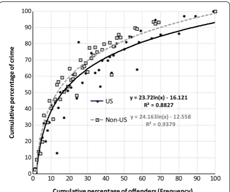
We calculated the prevalence curves using 95 data points from 10 studies that used data collected in the United States and 59 data points from 5 studies that used data from other countries. We calculated the frequency curves using 170 data points from 17 studies on the United States and 118 data points from 10 non-United States studies. In Figs. 7 and 8, the solid lines represent the United States curves and the dashed lines represents the non-United States curves. The comparison of the curves in Fig. 7 shows little difference in the prevalence of offending between the United States and other coun-tries. The 10% of people who are most involved in crime in the United States account for about 63% of the crime, whereas the same 10% in other nations account for 68% of crime, and the difference between the curves’ stand-ard errors is also small. Thus, our results suggest that Fig. 5 Male and female offending prevalence
the prevalence of offending does not vary substantially between nations. The curves in Fig. 8 also show some difference in offending frequency. Offending appears to be slightly less concentrated in the United States than in other countries. Our results suggest that repeat offend-ing is somewhat more widespread among offenders in the United States than among offenders in other nations, but the differences between the curves are small (particularly in their leftmost portions). These results seem to be con-sistent with the pattern in Rocque et al.’s (2015b) findings. In other words, there is some variation in the concentra-tion of offending between naconcentra-tions, but these differences are not substantial, and the greater amount of spread we
observe in the United States data points may be due to variations in the methods used in those studies.
Comparison to crime concentration “standards”
There are several concentration benchmarks in the lit-erature. These “standard” statistics include: (1) the worst 5% of a population (e.g., Weisburd 2015; Weisburd et al. 2004); (2) the worst 10% of offenders (e.g., Eck 2001; Spelman 1986; Spelman and Eck 1989); and (3) the worst 20% of offenders (e.g., Clarke and Eck 2005; Koch 1998). These serve as points of similarity between ours and other concentration studies that we can use to compare our results (see Appendix B for a detailed list of these sta-tistics for each our comparisons).
The “worst 5%” is a crime concentration statistic often associated with places and crime in the environmen-tal criminology literature. For example, Weisburd et al. (2004) found that about 5% of street segments in Seat-tle generated about 50% of the city’s police incident reports. Although this study focused on crime concen-tration among a population of places, recall that Wolf-gang et al.’s (1972) chronic offenders represented 6% of the entire 1945 Philadelphia birth cohort and accounted for 51.6% of all its offenses. In our prevalence compari-sons, we found that in the overall analysis and among youths, adults, males, and nations, 5% of each population accounted for between about 47 and 55% of crime. The concentration of crime was lower among females, with 5% of all females accounting for about 43% of crimes.
Recall that Spelman (1986) found that the worst 10% of offenders accounted for 40% of offenses. Spelman and Eck (1989) later suggested that crime was even more concentrated among this group. They estimated that the worst 10% of offenders account for about 55% of offenses. Our overall frequency analysis shows that the worst 10% of offenders account for about 41% of crime, which is closer to the results from Spelman’s (1986) anal-ysis. Moreover, our results suggest that the worst 10% of offenders account for about 40% of crime in all of our comparisons. Across the overall, gender, age, and nation frequency comparisons, 10% of the worst offenders accounted for between 37 and 43% of offending.
The final statistic is the Pareto principle, which Italian economist Vilfredo Pareto discovered in 1897 to describe the mathematical relationship he observed between a given proportion of the population and the amount of wealth associated with those people. Pareto noted that a minority of individuals accounted for a disproportion-ate amount of wealth and that this relationship followed a consistent and predictable pattern (Koch 1998). The Pareto principle is often alternatively referred to in busi-ness and economics literature as the “80/20 principle,” meaning that 80% of a system’s outputs are due to only y = 24.269ln(x) + 7.5151
R² = 0.7951
y = 20.368ln(x) + 22.045 R² = 0.7886
0 10 20 30 40 50 60 70 80 90 100
0 10 20 30 40 50 60 70 80 90 100
Cu
mu
la
v
e
pe
rc
en
ta
ge
of
cr
im
e
Cumulave percentage of offenders (Prevalence) US
Non-US
Fig. 7 United States and non-United States offending prevalence
y = 23.72ln(x) - 16.121 R² = 0.8827 y = 24.163ln(x) - 12.558
R² = 0.9379
0 10 20 30 40 50 60 70 80 90 100
0 10 20 30 40 50 60 70 80 90 100
Cu
mu
la
v
e
pe
rc
en
ta
ge
of
cr
im
e
Cumulave percentage of offenders (Frequency)
US
Non-US
20% of its inputs (Koch 1998). However, the 80/20 princi-ple has been discussed in the environmental criminology literature as well (e.g., Andresen 2014; Clarke and Eck 2005; Weisburd et al. 2012).
In the context of offending, Clarke and Eck (2005) invoke the 80/20 principle and state that 20% of offend-ers account for 80% of crime. Looking again at the over-all frequency distribution, our results show that 20% of offenders account for about 58% of crime. Likewise, across our other frequency comparisons, 20% of offend-ers account for between 52 and 60% of crime. These results seem to suggest that offending is less concen-trated than other phenomena often described using the 80/20 principle. However, looking instead at the preva-lence of offending in the overall analysis and among youths, adults, males, and nations, 20% of each popula-tion accounts for between 79 and 83% of crime. Similar to our results regarding the worst 5% of the population, offending was somewhat less concentrated among the female offender group, with 20% of all females accounting for about 75% of crimes by women.
Discussion
Across our comparisons, crime was less concentrated among the offender-only groups (frequency) than among the populations of offenders and non-offenders (preva-lence). As we noted earlier, this was an expected result and serves at least to support the reliability of our analy-sis. Our most interesting findings were the results of the comparisons between different offender and population groups. For youths and adults, our findings question Hirschi and Gottfredson’s (1983) assumption that the prevalence and frequency of crime invariantly declines in early adulthood. If offending is less common in adult-hood than in adolescence, then we would expect the prevalence and frequency of crime among adults to be more concentrated. However, our results suggest that offending is equally prevalent between these two groups and that crime is equally distributed among the most frequent offenders. The finding that offending is simi-larly distributed between youth and adults supports the need for criminal career research and the examination of the factors that influence fluctuations in the patterns of offending from adolescence through adulthood. As Cul-len (2011) argues, criminology has long been the study of adolescent offending. However, the similarities ado-lescents share with adults in the distribution of offending suggest that adult offending should not be ignored in the development of crime prevention interventions.
Our gender analysis provided several findings that were inconsistent with the literature on female offenders. First, our results suggested that a greater proportion of females than males become involved in crime. Second, crime was
somewhat less concentrated among the worst 5 and 20% of female offenders compared to the same proportion of offenders in the other analysis groups (i.e., males, youths and adults, United States and other nations). One expla-nation for these unexpected results is that our female prevalence and frequency curves are based on only 17 and 35 cumulative data points, respectively. Having few studies and data points for female offending may have influenced our findings. In other words, if female offend-ing research was as common as male offendoffend-ing research, our results might be different. Compounding this poten-tial problem is the fact that the data points for females appear more dispersed around the female curve than the data points around the male curve (see Figs. 5, 6). Thus, we are less confident that our results are valid with respect to female offending.
Across nations, involvement in crime appears to be equally prevalent although the frequency of crime in the United States appears to be slightly less concentrated among its worst offenders. Our results seem to sup-port Rocque et al.’s (2015b) finding that offending varies across different cultural contexts, but also that this vari-ation is not large. However, the dichotomy we used to compare the United States and other nations obscures the differences between countries in the latter category and the potential influence of those differences on crime concentration.
Many of our results are also consistent with the 5, 10, and 20% markers commonly referenced in the crime con-centration literature. However, our findings do under-score the importance of considering crime concentration among populations rather than restricting analysis to offender groups only. For example, the Pareto principle has been cited in the environmental criminology litera-ture to predict that 20% of all offenders account for 80% of all crime. Based on our analysis, a more appropriate interpretation would be that 20% of all individuals in a population account for 80% of all crime (which is in line with Vilfredo Pareto’s original use of the principle).
Limitations
We based our conclusions on the decisions we made in conducting our systematic review of offending and defin-ing the inclusion criteria for our analysis. Thus, if another researcher conducted a similar review of the literature, but made different decisions at those stages, it is theo-retically possible that he or she would arrive at differ-ent results. Though we are confiddiffer-ent that our decisions are appropriate, their validity can only be assessed by replication.
finding (e.g., not reported in titles and abstracts, but found in tables and appendices as background informa-tion), it is possible that we missed some relevant stud-ies when conducting the systematic review. Moreover, we restricted our review to empirical studies written in English, which may have excluded some foreign language publications with relevant concentration statistics. Thus, our results should be regarded as tentative rather than conclusive statements on offending concentration.
Second, we excluded 43 studies from our analysis because they did not provide sufficient data points. One problem with excluding studies is that it limits the varia-tion our data and thus restricts the types of comparisons we can make. Although we were limited to overall, gen-der, age, and nation comparisons due to the character-istics of the studies we collected, these are not the only important comparisons to make about offenders.
Third, we used only a single functional form, a loga-rithmic curve, to describe all our distributions. This con-sistency helps us to make comparisons, but it necessarily assumes there is only one functional form to describe all these data when it is possible that different groups have different functional forms. For example, it is possible in principle that male offending follows a different func-tional form than female offending, though we know of no theory that would support such a claim.
Fourth, using visual binning to construct the loga-rithmic curves was our best option to aggregate the x–y ordered pairs for analysis, but in consequence, we may have lost some variation in our data. We acknowledge that with no precedent for this type of analysis, our meth-ods leave room for improvement. We believe we have made progress toward closing a gap in the crime pre-vention literature by expanding upon Spelman and Eck’s work, but we invite other researchers to join us in this achieving this goal.
Conclusions
This study is the first to systematically review the litera-ture on offending concentration and use a meta-analysis to synthesize the evidence. One of our reasons for doing
it was to assess whether the evidence collectively sup-ports what criminologists have long asserted: that crime is highly concentrated among a minority of offenders. Our findings suggest that these “wolves” are indeed a small and ravenous pack. Our results also lend support to practical strategies that focus their resources on the worst offenders to prevent the most crime. These find-ings seem obvious, but they are nevertheless important to highlight. The meta-analysis could have just as well suggested that our long-held assumptions about offend-ing concentration are wrong.
In this paper, we focused on addressing three questions. First, how concentrated is crime across all studies? Our results show that crime is highly concentrated among a small group of offenders, even in a heterogeneous distri-bution of crimes and offenders. Second, how much vari-ation exists among the worst offenders? We examined the variation in crime concentration among the worst 5, 10, and 20% of offenders across four different compari-sons. Except for females, we found that the distribution of offending within each group is similar at these points. Third, how does crime concentration compare across dif-ferent offender groups? We found few differences in the concentration of offending across the different groups we compared.
separate paper we compare crime concentration in these three domains to determine if Spelman and Eck’s findings are still valid (Eck et al. 2017).
Our findings suggest that the implications drawn from the most prominent studies in the literature are prob-ably sound: a few people do commit the most crimes, and among offenders, a relatively small group are responsible for most crimes. The policy implications we can draw are obvi-ous: focus attention on the most active offenders. For situ-ational crime prevention and related interventions, it may be worth considering why a few offenders find some targets and places very attractive, but most people, and most other offenders, do not. Do they perceive opportunities differ-ently, or are they more exposed to attractive opportunities? Environmental criminology-based prevention and policies often do not differentiate between high-frequency offenders and sporadic offending, but perhaps they should.
Authors’ contributions
This paper was conducted by a team. NNM was the lead writer for this paper, contributed to the development of the methods used, and provided expertise on offenders. YL was the lead analyst for the team and provided editorial assistance. JEE headed the team and provided overall guidance and editorial assistance. SO provided expertise on victims assisted in the development of the research methods, and provided editorial reviews. All authors read and approved the final manuscript.
Author details
1 School of Criminal Justice, University of Cincinnati, Cincinnati, OH 45221, USA. 2 School of Public Affairs, University of Colorado, Colorado Springs, CO 80918, USA.
Acknowledgements
Authors thank the reviewers for their useful comments.
Competing interests
The authors declare that they have no competing interests.
Availability of data and materials
Articles used in the systematic review are noted in the references. For other information regarding data, please contact the lead author.
Consent for publication
Not applicable.
Ethics approval and consent to participate
Does not apply. As a review of summary data from previously conducted research, no humans (or their tissues) participated as subjects in this research.
Funding
No funds were solicited or provided for this research.
Appendices
Appendix A: Estimated distributions of crime prevalence and frequency among offenders: a comparison of fitted lines between un‑weighted and weighted X–Y ordered pairs
0
y = 23.173ln(x) + 12.24 R² = 0.8384
y = 21.282ln(x) + 19.54 R² = 0.809
10 20 30 40 50 60 70 80 90 100
0 10 20 30 40 50 60 70 80 90 100
Cumu
la
v
e
pe
rc
en
ta
ge
of
cr
im
e
Cumulave percentage of offenders
Prevalence
Weighted Prevalence
y = 23.914ln(x) - 13.761 R² = 0.9231
y = 25.151ln(x) - 19.849 R² = 0.8509
0 10 20 30 40 50 60 70 80 90 100
0 10 20 30 40 50 60 70 80 90 100
Cumu
la
v
e
pe
rc
en
ta
ge
of
cr
im
e
Cumulave percentage of offenders Frequency
Weighted Frequency
Publisher’s Note
Springer Nature remains neutral with regard to jurisdictional claims in pub-lished maps and institutional affiliations.
Received: 17 February 2017 Accepted: 25 July 2017
References
* Denotes a study identified for the systematic review. †Denotes a study
included in the analysis.
*†Ambihapathy, C. (1983). Criminal career research in the city of Ottawa. (Unpub-lished doctoral dissertation). University of Ottawa, Canada.
Andresen, M. A. (2014). Environmental criminology: Evolution, theory, and prac-tice. New York, NY: Routledge.
Auerhahn, K. (1999). Selective incapacitation and the problem of prediction.
Criminology,37(4), 703–734.
Babinski, L. M., Hartsough, C. S., & Lambert, N. M. (2001). A comparison of self-report of criminal involvement and official arrest records. Aggressive Behavior,27, 44–54.
*Baker, L. A., Mack, W., Moffitt, T. E., & Mednick, S. (1989). Sex differences in prop-erty crime in a Danish adoption cohort. Behavior Genetics,19(3), 355–370. *Barnes, J. C. (2014). Catching the really bad guys: an assessment of the
effi-cacy of the US criminal justice system. Journal of Criminal Justice,42(4), 338–346.
*Beaver, K. M. (2011). Genetic influences on being processed through the criminal justice system: results from a sample of adoptees. Biological Psychiatry,69(3), 282–287.
*†Beaver, K. M. (2013). The familial concentration and transmission of crime.
Criminal Justice and Behavior,40(2), 139–155.
*†Beck, A. J., & Shipley, B. E. (1987). Recidivism of young parolees. Washington, DC: US Department of Justice, Bureau of Justice Statistics. Beel, J., & Gipp, B. (2009). Google Scholar’s ranking algorithm: an
introduc-tory overview. In B. Larsen & J. Leta (Eds.), Proceedings of the 12th
International Conference on Scientometrics and Informetrics (Vol. 1, pp. 230–241).
*Block, C. R., Blokland, A. A., van der Werff, C., van Os, R., & Nieuwbeerta, P. (2010). Long-term patterns of offending in women. Feminist Criminol-ogy,5(1), 73–107.
Blumstein, A., Cohen, J., & Farrington, D. P. (1988). Criminal career research: Its value for criminology. Criminology,26, 1–35.
*†Brame, R., Fagan, J., Piquero, A. R., Schubert, C. A., & Steinberg, L. (2004). Criminal careers of serious delinquents in two cities. Youth Violence and Juvenile Justice,2(3), 256–272.
*Brame, R., Mulvey, E. P., Piquero, A. R., & Schubert, C. A. (2014). Assessing the nature and mix of offences among serious adolescent offenders. Crimi-nal Behaviour and Mental Health,24(4), 254–264.
*Brennan, P., Mednick, S., & John, R. (1989). Specialization in violence: Evidence of a criminal subgroup. Criminology,27(3), 437–453.
*Brennan, P. A., Mednick, S. A., & Hodgins, S. (2000). Major mental disorders and criminal violence in a Danish Birth Cohort. Archives of General Psychiatry, 57, 494–500.
*Caicedo, B., Gonçalves, H., González, D. A., & Victora, C. G. (2010). Violent delinquency in a Brazilian birth cohort: The roles of breast feeding, early poverty and demographic factors. Paediatric and Perinatal Epidemiology, 24(1), 12–23.
*Carkin, D. M. (2014). Criminal career paths in the 1958 Philadelphia birth Cohort: Onset, progression, and desistance (Unpublished doctoral dissertation). University of Massachusetts, Lowell.
*†Carrington, P. J., Matarazzo, A., & DeSouza, P. (2005). Court careers of a
Cana-dian birth cohort. Ottawa: Canadian Centre for Justice Statistics. *Cernkovich, S. A., Giordano, P. C., & Pugh, M. D. (1985). Chronic offenders: The
missing cases in self-report delinquency research. Journal of Criminal Law & Criminology,76, 705–732.
Clarke, R. V. G. (Ed.). (1997). Situational crime prevention. Monsey, NY: Criminal Justice Press.
Clarke, R. V. (2004). Technology, criminology, and crime science. European Journal on Criminal Policy and Research,10(1), 55–63.
Clarke, R. V., & Eck, J. E. (2005). Crime analysis for problem solvers. Washington, DC: Center for Problem Oriented Policing.
Table 2 Estimated coefficients and summary statistics of the model specifications in Figs. 1, 2, 3, 4, 5, 6, 7, 8
Figure number Key N study N (X, Y) Constant Beta Std. error Confidence
interval t‑statistic Percentage of crime explained by 5% 10% 20% 50%
Figure 1 Full prevalence 15 154 12.24 23.17 1.67 19.83 26.52 13.86 49.5 65.6 81.7 100.0 Partial prevalence 55 263 30.26 17.82 1.30 15.23 20.42 13.73 58.9 71.3 83.6 100.0 Full frequency 27 288 −13.76 23.91 0.87 22.17 25.65 27.50 24.7 41.3 57.9 79.8 Partial frequency 44 358 −13.23 24.17 0.95 22.27 26.08 25.36 25.7 42.4 59.2 81.3
Figure 2 Prevalence 15 154 12.24 23.17 1.67 19.83 26.52 13.86 49.5 65.6 81.7 100.0
Frequency 27 288 −13.76 23.91 0.87 22.17 25.65 27.50 24.7 41.3 57.9 79.8
Figure 3 Adult (P) 3 34 12.70 22.17 2.63 16.92 27.42 8.45 48.4 63.7 79.1 99.4
Youth (P) 7 64 7.67 23.80 2.75 18.30 29.30 8.65 46.0 62.5 79.0 100.0
Figure 4 Adult (F) 7 71 −7.61 21.20 1.11 18.98 23.42 19.09 26.5 41.2 55.9 75.3
Youth (F) 12 110 −17.01 23.56 1.67 20.22 26.90 14.12 20.9 37.2 53.6 75.2
Figure 5 Male (P) 13 108 12.04 23.33 1.68 19.97 26.69 13.90 49.6 65.8 81.9 100.0
Female (P) 5 17 6.12 22.95 3.59 15.77 30.13 6.39 43.1 59.0 74.9 95.9
Figure 6 Male (F) 14 119 −12.82 23.62 1.12 21.39 25.86 21.14 25.2 41.6 57.9 79.6
Female (F) 7 35 −13.73 22.06 3.78 14.50 29.63 5.83 21.8 37.1 52.4 72.6
Figure 7 US (P) 10 95 7.52 24.27 2.29 19.69 28.85 10.61 46.6 63.4 80.2 100.0
Non-US (P) 5 59 22.05 20.37 2.11 16.15 24.59 9.66 54.8 68.9 83.1 100.0
Figure 8 US (F) 17 170 −16.12 23.72 1.21 21.30 26.14 19.59 22.1 38.5 54.9 76.7
*Coid, J., Yang, M., Ullrich, S., Zhang, T., Roberts, A., Roberts, C., et al. (2007). Pre-dicting and understanding risk of re-offending: The prisoner cohort study. London: Ministry of Justice.
*†Collins, J. J. (1987). Some policy implications of sample arrest patterns. In M. E. Wolfgang, T. P. Thornberry, & R. M. Figlio (Eds.), From boy to man, delinquency to crime (pp. 76–86).
*†Collins, M. F., & Wilson, R. M. (1990). Automobile theft: Estimating the size of the criminal population. Journal of Quantitative Criminology,6(4), 395–409.
*Crowe, R. R. (1972). The adopted offspring of women criminal offenders: A study of their arrest records. Archives of General Psychiatry,27(5), 600–603.
Cullen, F. T. (2011). Beyond adolescence-limited criminology: Choosing our future—The American Society of Criminology 2010 Sutherland address.
Criminology,49(2), 287–329.
*Davis, M., Banks, S., Fisher, W., & Grudzinskas, A. (2004). Longitudinal patterns of offending during the transition to adulthood in youth from the men-tal health system. The Journal of Behavioral Health Services & Research, 31(4), 351–366.
*DeLisi, M. (2003). Criminal careers behind bars. Behavioral Sciences & the Law, 21(5), 653–669.
DeLisi, M., & Piquero, A. R. (2011). New frontiers in criminal careers research, 2000–2011: A state-of-the-art review. Journal of Criminal Justice,39(4), 289–301.
*DeLisi, M., & Scherer, A. M. (2006). Multiple homicide offenders: Offense characteristics, social correlates, and criminal careers. Criminal Justice and Behavior,33(3), 367–391.
*Denno, D. W. (1994). Gender, crime, and the criminal law defenses. The Journal of Criminal Law and Criminology,85(1), 80–180.
D’Unger, A. V., Land, K. C., & McCall, P. L. (2002). Sex differences in age patterns of delinquent/criminal careers: Results from Poisson latent class analy-ses of the Philadelphia cohort study. Journal of Quantitative Criminology, 18(4), 349–375.
Eck, J. E. (2001). Policing and crime event concentration. In R. F. Meier, L. W. Kennedy, & V. F. Sacco (Eds.), The process and structure of crime: Criminal events and crime analysis (pp. 249–276).
Eck, J. E., Clarke, R. V., & Guerette, R. T. (2007). Risky facilities: Crime concen-tration in homogeneous sets of establishments and facilities. Crime prevention studies (Vol. 21, pp. 225–264). Monsey, NY: Criminal Justice Press.
Eck, J. E., Lee, Y. J., O, S. H., & Martinez, N. N. (2017). Compared to what? Estimat-ing the relative concentration of crime at places usEstimat-ing systematic and other reviews. Crime Science, 6(8). doi:10.1186/s40163-017-0070-4 Edelstein, A. (2016). Rethinking conceptual definitions of the criminal career
and serial criminality. Trauma, Violence, & Abuse,17(1), 62–71. *†Elonheimo, H., Gyllenberg, D., Huttunen, J., Ristkari, T., Sillanmäki, L., &
Sourander, A. (2014). Criminal offending among males and females between ages 15 and 30 in a population-based nationwide 1981 birth cohort: Results from the FinnCrime Study. Journal of Adolescence,37(8), 1269–1279.
*Facella, C. A. (1983). Female delinquency in a birth cohort (Pennsylvania)
(Unpublished doctoral dissertation). University of Pennsylvania. Farrington, D. P. (1986). Age and crime. Crime and Justice,7, 189–250. Farrington, D. P. (1992). Criminal career research in the United Kingdom. The
British Journal of Criminology,32(4), 521–536.
Farrington, D. P. (2015). Cross-national comparative research on criminal careers, risk factors, crime and punishment. European Journal of Crimi-nology,12(4), 386–399.
*Farrington, D. P., Jolliffe, D., Hawkins, J. D., Catalano, R. F., Hill, K. G., & Koster-man, R. (2003). Comparing delinquency careers in court records and self-reports. Criminology,41(3), 933–958.
*Farrington, D. P., Jolliffe, D., Loeber, R., & Homish, D. L. (2007). How many offenses are really committed per juvenile court offender? Victims and Offenders,2(3), 227–249.
*†Farrington, D. P., & Maughan, B. (1999). Criminal careers of two London cohorts. Criminal Behaviour and Mental Health,9(1), 91–106. *Farrington, D. P., & West, D. J. (1990). The Cambridge study in delinquent
development: A long-term follow-up of 411 London males. Kriminalität
(pp. 115–138). New York, NY: Springer-Verlag.
*Farrington, D. P., & Wikstrom, P. O. H. (1994). Criminal careers in London and Stockholm: A cross-national comparative study. In E. G. M. Weitekamp
& H.-J. Kerner (Eds.), Cross-national longitudinal research on human devel-opment and criminal behavior (pp. 65–89). Boston, MA: Kluwer. *Fergusson, D. M., Lynskey, M. T., & Horwood, L. (1996). Alcohol misuse and
juvenile offending in adolescence. Addiction,91(4), 483–494. *Fischer, B., Medved, W., Kirst, M., & Rehm, J. (2001). Illicit opiates and crime:
Results of an untreated user cohort study in Toronto. Canadian Journal of Criminology,43, 197–217.
*Fisher, W. H., Roy-Bujnowski, K. M., Grudzinskas, A. J., Jr., Clayfield, J. C., Banks, S. M., & Wolff, N. (2006). Patterns and prevalence of arrest in a statewide cohort of mental health care consumers. Psychiatric Services,57(11), 1623–1628.
*Fry, L. J. (1985). Drug Abuse and crime in a Swedish birth cohort. British Jour-nal of Criminology,25(1), 46–59.
Gendreau, P. (1996). Offender rehabilitation: What we know and what needs to be done. Criminal Justice and behavior,23(1), 144–161.
*†Glueck, S., & Glueck, E. (1950). Unraveling juvenile delinquency. Cambridge, MA: Harvard University Press.
*Graham, J. & Bowling, B. (1995). Young people and crime. Research Study, 145 London, UK: Home Office.
Greenwood, P. W., & Abrahamse, A. F. (1982). Selective incapacitation. Santa Monica, CA: Rand Corporation.
Guttridge, P., Gabrielli, W. F., Jr., Mednick, S. A., & Van Dusen, K. T. (1983). Criminal violence in a birth cohort. In K. T. Van Dusen & S. A. Mednick (Eds.),
Prospective studies of crime and delinquency (pp. 211–224). Boston, MA: Kluwer-Nijhoff.
*Haas, H., Farrington, D. P., Killias, M., & Sattar, G. (2004). The impact of different family configurations on delinquency. British Journal of Criminology, 44(4), 520–532.
*†Hamparian, D., Schuster, R., Dinitz, S., & Conrad, J. P. (1978). The violent few. Lexington, MA: DC Heath.
*Hamparian, D. M., Davis, J. M., Jacobson, J. M., & McGraw, R. E. (1985). The young criminal years of the violent few. Washington, DC: Department of Justice.
*†Harer, M. D. (1995). Recidivism among federal prisoners released in 1987.
Journal of Correctional Education,46(3), 98–128.
Hirschi, T., & Gottfredson, M. (1983). Age and the explanation of crime. Ameri-can Journal of Sociology,89(3), 552–584.
*Høgh, E., & Wolf, P. (1983). Violent crime in a birth cohort: Copenhagen 1953–1977. In K. T. Van Dusen & S. A. Mednick (Eds.), Prospective studies of crime and delinquency (pp. 249–267). Boston, MA: Kluwer-Nijhoff. *Juon, H. S., Doherty, E. E., & Ensminger, M. E. (2006). Childhood behavior and
adult criminality: Cluster analysis in a prospective study of African Americans. Journal of Quantitative Criminology,22(3), 193–214. *Kempf-Leonard, K., Tracy, P. E., & Howell, J. C. (2001). Serious, violent, and
chronic juvenile offenders: The relationship of delinquency career types to adult criminality. Justice Quarterly,18(3), 449–478.
Kirk, D. S. (2006). Examining the divergence across self-report and official data sources on inferences about the adolescent life-course of crime. Journal of Quantitative Criminology,22(2), 107–129.
Koch, R. (1998). The 80/20 principle. New York, NY: Doubleday.
Lee, Y. J., Eck, J. E., O, S. H., & Martinez, N. N. (2017). How concentrated is crime at places? A systematic review from 1970 to 2015. Crime Science, 6(6). doi:10.1186/s40163-017-0069-x.
Lilly, J. R., Cullen, F. T., & Ball, R. A. (2015). Criminological theory: Context and consequences (6th ed.). Los Angeles, CA: Sage.
*†Liu, J., Messner, S. F., & Liska, A. E. (1997). Chronic offenders in China.
Interna-tional Criminal Justice Review,7(1), 31–45.
Lowenkamp, C. T., & Latessa, E. J. (2004). Understanding the risk principle: How and why correctional interventions can harm low-risk offenders. Topics in Community Corrections,2004, 3–8.
*Mazerolle, P., Brame, R., Paternoster, R., Piquero, A., & Dean, C. (2000). Onset age, persistence, and offending versatility: Comparisons across gender.
Criminology,38(4), 1143–1172.
*†Mednick, S. A., Gabrielli, W. F., & Hutchings, B. (1984). Genetic influences in criminal convictions: Evidence from an adoption cohort. Science, 224(4651), 891–894.
*†Nevares, D., Wolfgang, M. E., Tracy, P., & Aurand, S. (1990). Delinquency in
Puerto Rico. London: Greenwood Press.