of Population Mean in Two-Phase Sampling
L.N. Sahoo
Department of Statistics, Utkal University Bhubaneswar 751004, India
B.C. Das
Department of Statistics, Utkal University Bhubaneswar 751004, India
S. C. Senapati
Department of Statistics, Ravenshaw College Cuttack 753003, India
Summary
The present paper deals with the estimation of a finite population mean in the presence of two auxiliary variables under a two-phase sampling set up. It is assumed that the population mean of one auxiliary variable is known while that of other is unknown. Using the concept of predictive estimation developed by Basu (1971), a general class of estimators has been proposed. Analytical as well as simulation studies have been undertaken for evaluating performance of the suggested class.
Keywords & Phrases: Asymptotic variance, Auxiliary variable, Predictive approach, Two-phase sampling.
AMS 1991 Subject Classification: 62D05.
1. Introduction
Let yi,xi and zi (1i N) be the values of the study variabley and two auxiliary variables x and z respectively for the ith unit of a finite population U with means
N
i i
y N Y
1
1 ,
N
i i
x N X
1
1 and
N
i i
z N Z
1
1 . Suppose that X is unknown but Z is
known and our aim is to estimate Y from a random sample obtained through a two-phase selection. Allowing simple random sampling without replacement (SRSWOR) in each phase, we consider a two-phase sampling: At phase one, a sample s(sU)of nunits
is drawn from U to observe x and z. Then a sub-sample s (s s) of n units is drawn from sat the second phase to observe y only. Let us define
s
i i
y
y ,
s i i
x n
x 1 ,
s i i
z n
z 1 ,
s
i i
x n
x 1 and
s i i
z n
The basic work on estimation in this area was initiated by Chand (1975) and subsequently studied by Kiregyera (1980, 1984) among others. But, Sahoo and Sahoo (1993), Singh et al.(1994) and Sahoo and Sahoo (1999) developed three different classes of estimators for
Y defined by g
y,x,g(x,z)
, Z z x x y pp , ,
and q
q(y,x),x,z
respectively, such that various functions considered for composing of the classes satisfy certain regularity conditions. However, an analysis of the properties of these classes clearly shows that they are not necessarily disjoint, but attain the same asymptotic minimum variance bound (MVB), given by
) ( min ) ( min ) (
minV g V p V q
2 2
22 ( )(1 ) (1 )
y yz
yx C
Y
, (1)
where N n 1 1 , N n 1 1
, Cy is the coefficient of variation of y; yxand yzare respectively the correlation coefficients between y,x and y,z. An estimator attaining this MVB (may be called as an MVB estimator) is a regression-type estimator
) (
)
(x x b z Z b
y yx yz
RG
,
considered earlier by Sahoo et al. (1994), where byxand byz are respectively the sample regression coefficients of y on x and y on z computed using data available on s.
p g
, and q are also more efficient than y (y,x,x), a two-phase sampling
extension of Srivastava’s (1980) class of estimators, in respect of MVB criterion. It may be mentioned here that the MVB of y and the resulting MVB estimator are given by
2
22 ( )(1 ) )
(
minV y Y yx Cy (2) and
), (x x b
y
yRG yx
the classical two-phase sampling regression estimator of Y .
In this paper, we utilize the same available information on both auxiliary variables as have been used to compose g or p or q and construct a general class of estimators adopting the prediction criterion given by Basu (1971, p. 212, example 3).
2. Prediction Criterion in Two-Phase Sampling
Decomposing U into three mutually exclusive domains s, r2 ss and r1 Us
of n, nn and Nn units respectively, where s U s denotes the collection of
units in U which are not included in s, it is possible to express
s
i yi i r yi i r yi
N Y
2 1
1 . (3)
Writing
2 2 ) ( r i i y Y nn and
1 1 ) ( r i i y Y n
N , we have
1 2 (1 )
)
(f f Y f Y
y f
where
N n f and
N n
f . The first component of the right hand side of (4) is exactly
known. Hence, predicting unknown quantities Y1 and Y2 by T1 and T2 respectively on
the basis of sample data, a predictor Yˆ of Y can be represented by the equation
1 2 (1 )
) (
ˆ fy f f T f T
Y . (5)
It may be noted here that whenssU , Yˆ Y which is the target of our prediction.
For different choices of the predictors, the predictive equation (5) generates a family of estimators. Accordingly, considering T1 yZ1/z and T2 yX2/x, where
n n
x n x n X
2 and Z NNZ nnz
1 , Sahoo and Sahoo (2001) developed a ratio-type
estimator defined by
z Z y y y f
l1R ( R ) ,
where
x x y yR
, the classical two-phase sampling ratio estimator. On the other hand,
considering T1 ybyz(zZ1) and T2 ybyx(xX2), Sahoo et al. (2003) obtained
a regression-type estimator
). (
) (
1 y fb x x b z Z
lRG yx yz
The authors also derived sufficient conditions for the superiority of l1R and l1RG over the estimators
z Z x x
y
11
,
proposed by Chand (1975), and
( )
22 ybyx x xbxz zZ
,
proposed by Kiregyera (1984), where bxz is the sample regression coefficient of x on z based on s.
3. The Proposed Class of Estimators
For given s and s, let t1 (y,z,Z1) and t2 (y,x,X2,z,Z2),where
n n
z n z n Z
2 ,
assume values in R3 and R5, the 3- and 5-dimensional real spaces containing the points
) , , (
1 Y Z Z
and 2 (Y,X,X,Z,Z) respectively. Further, let h1(t1) and h2(t2) be
some known functions of t1 and t2 respectively such that h1(1)h2(2)Y. Further
assume that,
(a) the functions h1 and h2 are continuous in R3 and R5 respectively, and
Thus, based on information available on zin the domain r1, h1(t1) clearly defines a class
of estimators for Y. Similarly, availing information on both xand zin the domain r2, )
( 2
2 t
h also defines a class of estimators for Y . Hence, substituting T1 h1(t1) and )
( 2
2 2 h t
T in (5), we now define the following class of predictive estimators for Y : ). ( ) 1 ( ) ( )
(f f h2 t2 f h1 t1 y
f
lh
Note that when sU and z is not involved, our result corresponds to single phase
samplingi.e., selection of s fromUby SRSWOR with one auxiliary variablex. Then we have ), , , ( ) 1
( f h2 y x X2
y f
lh
which defines a class of estimators of Y . On the other hand, if no auxiliary information is taken into account, h1 h2 y,which implies that lh y, the simple expansion estimator of Y.
Many estimators of Y using x and z may turn out as particular cases of lh. For example, ,
1R
l 11,l1RG and 22are particular cases of lhfor some specific selections of h1and h2.
However, we also consider the following two noteworthy cases: (i) Let
z Z y h 1
1 and h2 y Xx2 Zz2 , then
z Z y y y z z y f z z y y f l
lh R R R
2 (1 ) (1 ) ,
where . n n n
(ii) Let h1 ybyz(zZ1) and h2 ybyx(xX2)byz(zZ2), then ). ( ) ( ) (
2 y fb x x fb z z b z Z
l
lh RG yx yz yz
4. Asymptotic Variance of the Class
Expanding h1(t1)and h2(t2)around the points 1 and 2respectively in a first order
Taylor’s series and then neglecting the remainder terms, we get
) ( ) ( ) ( ) ( )
(1 1 1 11 12 13 1
1 t h h y Y h z Z h Z Z
h (6)
and ) ( ) ( ) ( )
( 2 2 2 21 22
2 t h h y Y h x X
h
) ( 2 23 X X
h
h24(zZ)h25(Z2 Z), (7)
where hij is the partial derivative of hi(ti) w.r.t. itsjth argument around the point i, i 1,2 ; j1,2,3,4,5. Further, noting that h11 h21 ,1h12 h13,h22 h23 and h24 h25,
we have after a considerable simplification
) ( ) ( ) ( )
(y Y fh22 x x fh24 z z h12 z Z
Y
This shows that the bias of lh is of order n1 and hence its contribution to the mean square error is of order n2.
From (8), after a few algebraic steps suppressed to save space, the asymptotic variance of h
l is obtained as
y x z yx yz xz
h S f h S f h S fh S fh S f h h S
l
V( )() 2 2 222 2 2 242 2 2 22 2 24 2 2 22 24
S2y h122Sz2 2h12Syz
, (9)
where ( ) ,
1
1 2
1
2 y Y
N
S N
i i
y
1 ( )( )
1 1
X x Y y N
S N i
i i
yx
etc. Hence,
) (lh
V attains
its minimum value when
0 22 .
22 / f h
h yxz (say)
0 24 .
24 / f h
h yzx (say)
and 0
12
12 h
h yz (say),
where yz is the regression coefficient of yon z; yx.z and yz.x are respectively the partial regression coefficients of y on x and y on z. The minimum value of V(lh) i.e., the asymptotic MVB of lh is given by
( )(1 ) (1 )
,) (
min 2 2 2
. 2
y yz xz
y
h Y C
l
V (10)
where y.xz is the multiple correlation coefficient of y on x and z. The corresponding MVB estimator is a regression-type estimator
), (
) ( )
( .
. x x b z z b z Z
b y
lRG yxz yzx yz
suggested by Tripathi and Ahmed (1995), where byx.z and byz.x are respectively sample partial regression coefficients of yon xand yon zbased on s.
4. Precision of the Class
Our objective is to study precision of the predictive method of estimation developed in this work compared to the classical method. For this we need to compare efficiency of lh with that of y,g,p and q. But, the task of drawing a meaningful conclusion by comparing all estimators belonging to two different classes is not easy. Because, an estimator has its own limitations and can also be suitable for a particular situation in terms of the relationship between the variables under consideration. However, for simplicity, here we concentrate on the MVB estimators only i.e., we accept MVB as a precision measure of a class. On the basis of this consideration, from (1), (2) and (10) we see that,
) ( min ) ( min ) (
minV lh V g V y
Hence, we conclude that on the ground of MVB, the class of estimators represented by lh is definitely superior to the classes of estimators represented by y and g or p or q. To study efficiency of some specific predictive estimators belonging to lh compared to some similar type of classical estimators belonging to y and g or p or q numerically, we have carried out a simulation study that involved repeated draws of random samples from the following populations:
Population I [Murthy (1977), p. 228]: Consists of data on output(y), number of workers(x) and fixed capital(z)for 80 factories. We consider n= 20 and n= 10.
Population II [Sarndal, Swensson and Wretman (1992), p. 662]: Consists of data on 1983 import(y), 1983 population (x) and 1980 population (z) for 124 countries. We consider n= 30 and n= 12.
5000 independent first phase samples each of size nwere selected from a population by
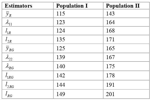
SRSWOR. Then, from each selected first phase sample, a second phase sample of size n was again selected by SRSWOR. For each combination(n,n), values of several estimators were computed. Then, considering 5000 such combinations simulated mean square errors of the estimators were calculated. Relative efficiencies of different estimators compared to the expansion estimator y are displayed in table 1.
From table 1 it is observed that lRG attains the maximum precision and the suggested regression-type estimator l2RG has better precision than other predictive and non-predictive estimators. The suggested ratio-type estimator l2R also leads to substantial increase in precision over other ratio and ratio-type estimators.
Table 1: Relative Efficiency of Different Estimatorsw.r.t. y(in) Estimators Population I Population II
R
y 115 143
11
123 164
R
l1 124 168
R
l2 135 171
RG
y 125 165
22
139 167
RG
140 175
RG
l1 142 178
RG
l2 144 191
RG
5. Conclusions
We have made a successful attempt in constructing a class of estimators for the finite population mean that is decidedly better than some other classes gathering information on two auxiliary variables in a two-phase sampling. Because, our analytical comparison shows that the suggested class is more efficient than others on the ground of MVB criterion. On the other hand, from the simulation study it is also seen that some estimators of the proposed class are more efficient than some similar type estimators belonging to other classes. These findings clearly indicate that there are situations which can favor for the application of the suggested estimation methodology. Of course, our analytical and simulation studies have limited scope and cannot able to reveal essential features of different classes in a straightforward manner. Further investigations may be made for arriving at better conclusions.
References
1. Basu, D. (1971). An essay on the logical foundations of survey sampling, Part I.
Foundations of Statistical Inferences, V.P. Godambe and D.A. Sprott (eds), Holt, Rinehart and Winston, Toronto, Canada, 203-204.
2. Chand, L. (1975). Some Ratio-type Estimators Based on Two or More Auxiliary Variables. Unpublished Ph.D. Dissertation, Iowa State University, Ames, Iowa. 3. Kiregyera, B. (1980). A chain ratio-type estimator in finite population double
sampling using two auxiliary variables. Metrika, 27, 217-223.
4. Kiregyera, B. (1984). Regression-type estimators using two auxiliary variables and the model of double sampling from finite populations.Metrika, 31, 215-226. 5. Muthy, M.N. (1977). Sampling Theory and Methods. Statistical Publishing
Society, Calcutta.
6. Sahoo, J. and Sahoo, L.N. (1993). A class of estimators in two-phase sampling using two auxiliary variables. Jour. Indian Stat Assoc., 31, 107-114.
7. Sahoo, J. and Sahoo, L.N. (1999). An alternative class of estimators in double sampling procedures.Calcutta Stat. Assoc. Bull., 49, 79-83.
8. Sahoo, J. Sahoo, L.N. and Mohanty, S. (1994). An alternative approach to estimation in two-phase sampling using two auxiliary variables. Biometrical Jour., 36, 293-298.
9. Sahoo, L.N. and Sahoo, R.K. (2001). Predictive estimation of finite population mean in two-phase sampling using two auxiliary variables. Jour. Indian Soc. Agric. Stat., 54, 250-254.
10. Sahoo, L.N., Sahoo, R.K. and Senapati, S.C. (2003). Predictive estimation of finite population mean using regression-type estimators in double sampling procedures.Jour. Stat. Res., 37, 291-296.
12. Singh, V.K., Singh, Hari P., Singh, Housila P. and Shukla, D. (1994). A general class of chain estimators for ratio and product of two means of a finite population.
Comm. Stat. – Thoe. Meth., 23, 1341-1355.
13. Srivastava, S.K. (1980). A class of estimators using auxiliary information in sample surveys.Canad. Jour. Stat., 8, 253-254.