Surface solar irradiance from SCIAMACHY measurements: algorithm and validation

www.atmos-meas-tech.net/4/875/2011/ doi:10.5194/amt-4-875-2011

© Author(s) 2011. CC Attribution 3.0 License.

Measurement

Techniques

Surface solar irradiance from SCIAMACHY measurements:

algorithm and validation

P. Wang1, P. Stammes1, and R. Mueller2

1_{Royal Netherlands Meteorological Institute (KNMI), De Bilt, The Netherlands}

2_{Climate Monitoring Satellite Application Facility, German Meteorological Service (DWD), Offenbach, Germany} Received: 14 December 2010 – Published in Atmos. Meas. Tech. Discuss.: 2 February 2011

Revised: 29 April 2011 – Accepted: 9 May 2011 – Published: 16 May 2011

Abstract. Broadband surface solar irradiances (SSI) are,

for the first time, derived from SCIAMACHY (SCanning Imaging Absorption spectroMeter for Atmospheric Cartog-rapHY) satellite measurements. The retrieval algorithm, called FRESCO (Fast REtrieval Scheme for Clouds from the Oxygen A band) SSI, is similar to the Heliosat method. In contrast to the standard Heliosat method, the cloud in-dex is replaced by the effective cloud fraction derived from the FRESCO cloud algorithm. The MAGIC (Mesoscale Atmospheric Global Irradiance Code) algorithm is used to calculate clear-sky SSI. The SCIAMACHY SSI product is validated against globally distributed BSRN (Baseline Surface Radiation Network) measurements and compared with ISCCP-FD (International Satellite Cloud Climatology Project Flux Dataset) surface shortwave downwelling fluxes (SDF). For one year of data in 2008, the mean difference be-tween the instantaneous SCIAMACHY SSI and the hourly mean BSRN global irradiances is−4 W m−2(−1 %) with a standard deviation of 101 W m−2(20 %). The mean differ-ence between the globally monthly mean SCIAMACHY SSI and ISCCP-FD SDF is less than−12 W m−2(−2 %) for ev-ery month in 2006 and the standard deviation is 62 W m−2 (12 %). The correlation coefficient is 0.93 between SCIA-MACHY SSI and BSRN global irradiances and is greater than 0.96 between SCIAMACHY SSI and ISCCP-FD SDF. The evaluation results suggest that the SCIAMACHY SSI product achieves similar mean bias error and root mean square error as the surface solar irradiances derived from po-lar orbiting satellites with higher spatial resolution.

Correspondence to: P. Wang ([email protected])

1 Introduction

Information on surface solar radiation is relevant for a bet-ter understanding of climate change and global hydrological cycle, and for more efficient utilization of solar energy. Sci-entists have attempted to derive surface solar radiation from both geostationary and polar-orbiting satellite measurements. Various algorithms have been developed to produce surface solar radiation data sets based on radiative transfer calcula-tions and statistics (e.g. Moeser and Raschke, 1984; Cano et al., 1986; Bishop and Rossow, 1991; Pinker and Laszlo, 1992; Darnell et al., 1988; Li et al., 1993; Pinker et al., 2003; Zhang et al., 2004; Rigollier et al., 2004; Mueller et al., 2009; Wang and Pinker, 2009). The Pinker-Laszlo (1992) algo-rithm is used in the GEWEX (Global Energy and Water Cy-cle Experiment) Surface Radiation Budget Project to gener-ate the shortwave radiative fluxes (http://gewex-srb.larc.nasa. gov/). This approach has also been the basis for the first operational version of the EUMETSAT CM-SAF (Satellite Application Facility on Climate Monitoring) scheme (Holl-mann et al., 2006). The FRESCO (Fast REtrieval Scheme for Clouds from the Oxygen A band) SSI (Surface Solar Irradi-ance) algorithm that is presented in this paper uses a similar approach to the clear-sky approach of the new operational CM-SAF surface solar irradiance algorithm (Mueller et al., 2009). Therefore, some detailed introductions are provided for the Pinker-Laszlo algorithm and the new CM-SAF sur-face solar irradiance algorithm.

876 P. Wang et al.: Surface solar irradiance from SCIAMACHY measurements: algorithm and validation by ozone and water vapor, multiple scattering by molecules,

multiple scattering by aerosols and clouds, and multiple re-flections between the surface and the atmosphere.

The new operational CM-SAF surface solar irradiance al-gorithm is based on radiative transfer calculations and using satellite-derived parameters as input (Mueller et al., 2009). The radiative transfer calculations are characterized by the combination of parameterizations and eigenvector look-up tables. The clear-sky approach in the CM-SAF algorithm is comparable to the Mesoscale Atmospheric Global Irradiance Code (MAGIC) algorithm (see Sect. 2.3). The cloudy sky ap-proach in the CM-SAF algorithm relates the top of the atmo-sphere (TOA) albedo derived from the Geostationary Earth Radiation Budget (GERB) instrument to the surface irradi-ance. In order to calculate the surface solar irradiance using the TOA albedo, a sophisticated hybrid LUT approach is ap-plied and knowledge of the surface albedo and a cloud mask are needed. The cloudy part of this algorithm employs the additional spectral channels of the Meteosat Second Gener-ation (MSG) satellites. However, the algorithm is not suited to be applied to Meteosat First Generation (MFG). For MFG the CM-SAF algorithm uses the Heliosat method to consider the effect of clouds on the surface solar irradiance.

The Heliosat method was originally described by Cano et al. (1986). Later, various modifications have been made to improve the cloud index calculations (see Sect. 2.1.2) and the clear-sky model (Hammer et al., 2003; Rigollier et al., 2004; Mueller et al., 2004; Dagestad and Olseth, 2007). The basic idea of the Heliosat method is that the cloud index retrieved from satellite reflectances provides sufficient information to estimate the effect of clouds on the surface solar irradiance. After the retrieval of cloud index in the first step of the He-liosat method, the surface solar irradiance is derived by the use of a clear-sky model in a second step. The cloud index (n) is determined from the normalized reflectance. The clear-sky index (k) is the ratio between the actual (full-sky) surface solar irradiance (G) and the clear-sky surface solar irradi-ance (Gclr), namely,k=G/Gclr. The clear-sky surface solar irradiances calculated by the clear–sky model are converted into the full-sky surface solar irradiances using then−k rela-tion. In contrast to the CM-SAF method applied to MSG, the Heliosat method only uses the satellite derived reflectances for the cloud information while the surface albedo and cloud mask are not needed. The advantage of the Heliosat method is its capability to retrieve surface solar irradiance in high ac-curacy across Meteosat satellite generations. Moreover, the consistent treatment of the surface albedo effect (clear-sky reflectance) reduces the uncertainty arising from the usage of external surface albedo information and does not require the application of an angular distribution model, which is in turn an additional error source.

Different Heliosat algorithms were developed to pro-duce surface solar irradiance data sets from the Meteosat (MFG and MSG) measurements. These data sets have been extensively validated against ground-based solar radiation

measurements (Perez et al., 2001; Meyer et al., 2003; Rigol-lier et al., 2004). The relative standard deviation between hourly mean surface solar irradiances derived using the He-liosat algorithms and ground-based measurements is typi-cally 20–25 % (Ineichen and Perez, 1999; Zelenka et al., 1999; Dagestad, 2004; Lorenz, 2007). It is now well estab-lished that the surface solar irradiances derived from satel-lite measurements can be more accurate than those found by interpolation using ground-based measurements which are more than 30 km apart (Perez et al., 1997; Zelenka et al., 1999).

The Heliosat method has been mainly applied to the Me-teosat geostationary satellite measurements, which have the advantage of high spatial and temporal resolution. However, the Meteosat satellites do not provide global coverage but are restricted to a specific part of the world, covering Eu-rope and Africa. Global coverage, including the polar re-gions, is given by sun-synchronous polar orbiting satellites. SCIAMACHY (SCanning Imaging Absorption spectroMeter for Atmospheric CHartographY) is a spectrometer on board the Envisat satellite which flies in a sun-synchronous polar orbit with equator crossing time at about 10:00 LT (Local Time). Therefore, we adapted the Heliosat method to the SCIAMACHY measurements. The pixel size of the SCIA-MACHY nadir measurements is 60×30 km2and global cov-erage takes 6 days. The wavelength range of SCIAMACHY is from ultraviolet to near infrared with about 0.2–1.5 nm spectral resolution. The primary mission objective of SCIA-MACHY is global measurements of trace gases in the tropo-sphere and in the stratotropo-sphere, such as ozone, nitrogen diox-ide, water vapor, methane and carbon monoxide (Bovens-mann et al., 1999).

Cloud and aerosol information is required in the trace gas retrievals; therefore, several cloud retrieval algorithms have been developed for SCIAMACHY based on oxygen A band spectra measurements (e.g. Koelemeijer et al., 2001; Kokhanovsky et al., 2006) and based on the PMD (Polar-ization Measurement Device) measurements (e.g. Loyola, 2004; Grzegorski et al., 2006). The FRESCO cloud algo-rithm was first developed by Koelemeijer et al. (2001) to derive effective cloud fraction and cloud pressure and was improved by Wang et al. (2008) with the addition of sin-gle Rayleigh scattering (called FRESCO+ or FRESCO v5). In the FRESCO SSI algorithm, the effective cloud fraction is converted to surface solar irradiance using the Heliosat method and using the MAGIC algorithm (Mueller et al., 2004, 2009) for the clear-sky surface solar irradiances.

1

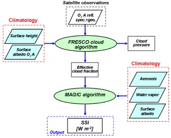
Figure 1. Flowchart of the FRESCO surface solar irradiance (SSI) algorithm.

2

3

Figure 2. Ratio of the effective cloud fractions retrieved with cloud albedo of 0.95 (c

)

4

and cloud albedo of 0.8 (c

) as a function of surface albedo (black stars) and the 3

-5

order polynomial fit

y

=

a

+

bx

+

cx

+

dx

(red line). The effective cloud fractions are

6

retrieved from the SCIAMACHY orbit over Europe, the Sahara desert and the Atlantic

7

Ocean on 4 February 2007 (orbit number 25785).

8

Fig. 1. Flowchart of the FRESCO surface solar irradiance (SSI) algorithm.

2 FRESCO SSI algorithm

Similar to the Heliosat method (Cano et al., 1986; Hammer et al., 2003), the FRESCO SSI algorithm consists of three steps: (1) calculate the effective cloud fraction; (2) calculate the clear-sky index (k) using the Heliosatn−krelation; (3) cal-culate the clear-sky and full-sky surface solar irradiances us-ingkand the MAGIC algorithm. Because FRESCO SSI uses then−krelation, it is essential to demonstrate that the effec-tive cloud fraction value can be equivalent to the cloud index value. The flowchart of the FRESCO SSI algorithm is shown in Fig. 1.

2.1 Calculation of effective cloud fraction 2.1.1 FRESCO cloud retrieval algorithm

In the FRESCO cloud algorithm, the independent pixel ap-proximation is used to account for partly cloudy pixels. In order to simulate the reflectance spectrum of a partly cloudy pixel inside and outside the O2A band, a simple atmospheric model is used, in which the atmosphere above the ground surface (for the clear-sky part of the pixel) or cloud (for the cloudy part of the pixel) is treated as an absorbing (due to oxygen) and purely Rayleigh scattering medium. Reflection occurs only at the surface and the cloud top. The surface and cloud are assumed to be Lambertian reflectors. The re-flectanceRsim(λ,θ,θ0,φ−φ0) at a wavelengthλ, viewing

zenith angleθ, solar zenith angle (SZA)θ0, and relative az-imuth angleϕ−ϕ0is then given by

Rsim (λ, θ, θ0, ϕ −ϕ0) = c TcAc +c Rc (1) +(1 −c) TsAs +(1 −c) Rs,

wherecis the effective cloud fraction,Acis the cloud albedo,

As is the surface albedo. T (λ,z,θ,θ0) is the direct atmo-spheric transmittance for light entering the atmosphere from the solar direction, propagating down to a level with surface heightzsor cloud heightzc, and then propagating to the top of the atmosphere in the direction of the satellite. The O2 absorption and single Rayleigh scattering are taken into ac-count in the light paths forT. The O2 line absorption pa-rameters are taken from the HITRAN 2004 database (Roth-man et al., 2005). Rc (λ,zc,θ, θ0,ϕ−ϕ0) andRs (λ, zs,

θ,θ0,ϕ−ϕ0) are the single Rayleigh scattering reflectances above the cloud and the surface, respectively (Wang et al., 2008). Tc,Ts, Rc, andRs are pre-calculated and stored in look-up tables. Because there is not enough independent information from the O2 A band to retrieve cloud fraction and cloud albedo simultaneously, in the FRESCO algorithm the cloud albedo is assumed as a fixed value for an optically thick cloud (Koelemeijer et al., 2001; Stammes et al., 2008).

Ac is assumed to be 0.8 when the effective cloud fraction is used for the trace gas retrieval (Koelemeijer et al., 2001). In the FRESCO SSI algorithm Ac is assumed to be 0.95 (see Sect. 2.1.2). Effective cloud fraction of a pixel means

878 P. Wang et al.: Surface solar irradiance from SCIAMACHY measurements: algorithm and validation the cloud fraction for a Lambertian cloud with a fixed cloud

albedo (of 0.8 or 0.95) which yields the same reflectance at the top of the atmosphere (TOA) as the real clouds in the pixel. The surface albedo (As) is taken from a monthly cli-matology (Koelemeijer et al., 2003). Surface height is from the GTOPO30 digital elevation model (http://eros.usgs.gov/ Find Data/Products and Data Available/gtopo30 info). The unknowns in Eq. (1) are c and zc. The reflectances at 15 wavelengths in the 758–759 nm, 760–761 nm, and 765– 766 nm bands are used in the retrieval. The retrieval method is based on minimizing the difference between the simulated and the measured spectra, using the Levenberg-Marquart nonlinear least-squares method.

2.1.2 Rationale of using effective cloud fraction as cloud index

Because the FRESCO SSI algorithm uses the Heliosatn−k

relation, the effective cloud fraction values have to be compa-rable to the cloud index values. As shown in Eq. (1), the re-trieved effective cloud fraction depends on the assumed fixed cloud albedo value. Therefore, the effective cloud fraction value can be similar to that of the cloud index by using a proper assumption for the fixed cloud albedo value.

In the Heliosat method, the cloud index (n) is defined as:

n = R −Rmin Rmax −Rmin

, (2)

whereR is the reflectance at the top of the atmosphere in the visible spectral channel, Rmax and Rmin are the corre-sponding maximum reflectance for the cloudy situation and the minimum reflectance for the clear-sky situation, respec-tively.Rmaxis usually selected as the 95–98 percentile of the reflectance at TOA (Hammer et al., 2003; Dagestad, 2004; Dagestad and Olseth, 2007). In order to calculate the cloud index, the reflectance at TOA has to be corrected for the ef-fects due to the surface reflection and the scattering of atmo-spheric molecules (Dagestad and Olseth, 2007).

By definingRcld=TcAc+RcandRclr=TsAs+Rs, accord-ing to Eq. (1) the effective cloud fraction can be calculated from:

c = Rsim −Rclr Rcld −Rclr

. (3)

Apparently Eq. (3) has the same form as Eq. (2). For the clear-sky situation, if the absorption in the atmosphere is neg-ligible,Rclr is dominated by the surface albedo and equiv-alent to Rmin. If Rcld is chosen similar to Rmax as well, the effective cloud fraction is defined in the same manner as the cloud index. At the continuum of the O2 A band, the Rayleigh scattering reflectance is about 0.02 at medium SZA andTc is close to 1. Therefore, the assumption ofAc to be 0.95 leads toRcldof 0.97, which is comparable to the 95–98 percentile of the reflectance. With this definition, the effective cloud fraction and the cloud index both express the

normalized reflectances to the optically thick clouds and their values are similar. Furthermore, the effective cloud fraction information is mainly obtained from the continuum of the O2 A band in the 758–759 nm wavelength range, which is within the visible spectral channel of Meteosat used originally to derive the cloud index. The wavelength differences of the effective cloud fraction and cloud index can be neglected. In principle, it is relatively simple and straightforward to re-place the cloud index with the effective cloud fraction and to use the established and validated Heliosat relation between cloud and clear-sky index, then−krelation.

2.2 Calculation of clear-sky index

As described in the introduction, the clear-sky index (k) is used to approximate the cloud transmission. When the cloud index is known, the clear-sky index can be calculated from then−krelation (Hammer et al., 2003). In the FRESCO SSI algorithm, the effective cloud fractioncis equal to the cloud indexnand always equal or greater than 0. Therefore,kis calculated using Eqs. (4)–(6):

0 ≤ n ≤ 0.8, k = 1 −n, (4)

0.8 < n ≤ 1.1, k = 2.0667−3.6667n+1.6667n2, (5)

1.1 < n, k = 0.05. (6)

The basic relation between the cloud index and the clear-sky index is defined by the law of energy conservation (Dages-tad, 2005) and based upon the observation that atmospheric transmission is linearly related to the earth’s planetary albedo (Schmetz, 1993). However, above a cloud index value of 0.8 an empirical adjustment has to be applied to correct for the non-linear behavior. The adjustment was determined from the statistical regression using ground-based measurements at European sites and fitted to get the best performance at all the ground sites. The close relationship of the Heliosat method to the law of energy conservation is probably the rea-son for the stability and “global” applicability of the Heliosat

n−krelation.

2.3 Calculation of surface solar irradiance

The surface solar irradiance for the full-sky situation (G) is given by,

G = k Gclr, (7)

model (RTM) results for aerosols with different aerosol op-tical thickness, single scattering albedo, and asymmetry pa-rameter values. Fixed values for water vapor, ozone and sur-face albedo have been used for the calculation of the basis LUT: 15 kg m−2for water vapor column, 345 DU of ozone, and a broadband surface albedo of 0.2. The effect of the so-lar zenith angle on the transmission, hence the surface soso-lar irradiance, is considered by the use of the Modified Lambert-Beer (MLB) function. The effects of variations in water va-por and surface albedo with respect to the fixed values used in the calculation of the basis LUT are corrected using correc-tion formulas and parameterizacorrec-tions (Mueller et al., 2009). The variation of ozone column amount is not taken into ac-count. The applied parameterizations have been derived by RTM calculations and are in line with explicit RTM results. The aerosol, water vapor and broadband surface albedo cli-matology databases in the MAGIC algorithm can be updated without changing the basis LUT and the code.

The sensitivities of the retrieved surface irradiance values to the variations of water vapor column amount, aerosol op-tical thickness and surface albedo have been analyzed by Mueller et al. (2009) and Wang et al. (2011). The surface solar irradiance shows a weak dependency on surface albedo for clear-sky cases (Mueller et al., 2009), e.g. a variation of the surface albedo of 50 % relative to a 0.2 reference value leads only to a variation of 1 % in clear-sky surface solar ir-radiance. The sensitivity of SSI to water vapor can be es-timated from Fig. 3 in Mueller et al. (2009). For example, if the water vapor column in the climatological database is 15 mm, but the actual water vapor column is 10 or 20 mm, the variation of SSI values is within +20 and−15 W m−2_. The effect of aerosol optical thickness (AOT) on the SSI is briefly discussed by Wang et al. (2011). For clear-sky cases, changes in AOT of±0.02 lead to changes in global irradiance of about±5.2 W m−2at cosine of solar zenith angle of 0.42. For fully cloudy cases (cloud optical thickness of 20.1), AOT changes of±0.02 cause changes in SSI of ±0.44 W m−2. Therefore, it is important to use proper aerosol, water vapor and broadband surface albedo data in the MAGIC algorithm. The input data of the MAGIC algorithm include: date, time, solar zenith angle, latitude, longitude, cloud index (ef-fective cloud fraction), water vapor column density, aerosol optical thickness and single scattering albedo, and broad-band surface albedo (see Fig. 1). The choice of water vapor, aerosol and broadband surface albedo data is discussed in Sect. 2.4. The output of the MAGIC algorithm is the clear-sky and full-clear-sky surface solar irradiances in the 0.2–4.0 µm wavelength region. The extraterrestrial total solar irradiance is 1365 W m−2 and is adjusted according to the Earth-Sun distance. Then−krelation is part of the MAGIC algorithm. The MAGIC algorithm is fast, robust and suitable for oper-ational applications. More details about the MAGIC algo-rithm are given by Mueller et al. (2004, 2009).

2.4 Configuration of the FRESCO SSI algorithm for SCIAMACHY

Within the ESA WACMOS (European Space Agency, Wa-ter Cycle Multi-mission Observation Strategy) project (Su et al., 2010), the surface solar irradiances in 2006 and 2008 have been derived from the SCIAMACHY measurements as a demonstration data set. The effective cloud fractions are taken from the TEMIS website directly, because the FRESCO cloud product from SCIAMACHY is one of the operational products from the ESA TEMIS (Tropospheric Emission Monitoring Internet Service, http://www.temis.nl) project. The FRESCO cloud product on the TEMIS web page is reprocessed using the latest version of SCIAMACHY Level 1 data. It is more efficient to use the existing effective cloud fraction than reprocessing the FRESCO cloud prod-uct using the SCIAMACHY Level 1 data. In the WACMOS project, we used the FRESCO data version sc-5.2 (Level 1 data v6.03). However, the fixed cloud albedo (in Eq. 1) is as-sumed to be 0.8 in the operational FRESCO cloud algorithm for the TEMIS project, because it leads to optimal effective cloud fractions for the trace gas retrievals (Koelemeijer et al., 2001; Stammes et al., 2008). In order to be consistent with the definition of the cloud index in the Heliosat method, the original FRESCO effective cloud fractions (c0.8) have to be converted to the effective cloud fractions with a fixed cloud albedo of 0.95 (c0.95), which gives the best performance for the SSI product. The conversion is carried out as follows. The FRESCO effective cloud fractionsc0.8 andc0.95 were retrieved by assuming the cloud albedo to be 0.8 and 0.95, respectively, for one SCIAMACHY orbit over Europe, the Sahara desert and Atlantic Ocean on 4 February 2007 (or-bit number 25785, measurement start time 10:30:03 UTC). The ratios of the two effective cloud fraction data sets were fitted as a function of the surface albedo (As) using a 3rd-order polynomial. The fit and the polynomial coefficients are shown in Fig. 2. According to the regression, c0.95 can be calculated from

c0.95 = c0.8

a +bx +cx2+dx3, (8) wherexis the averaged surface albedo at the O2A band. The fit to the SCIAMACHY data was checked with the fit derived from one full day (15 orbits) of GOME-2 (Global Ozone Monitoring Experiment) measurements and good agreement was found. As illustrated in Fig. 2, the fit is quite good ex-cept for a few outliers due to the cut off ofc0.8andc0.95at 1 (overcast situations for optically thick clouds). The outliers are not important, because SSI values are low in overcast situations with optically thick clouds. We have compared the SCIAMACHY SSI derived using the converted effective cloud fraction and the retrieved effective cloud fraction with

880 P. Wang et al.: Surface solar irradiance from SCIAMACHY measurements: algorithm and validation

41

1

Figure 1. Flowchart of the FRESCO surface solar irradiance (SSI) algorithm.

2

3

Figure 2. Ratio of the effective cloud fractions retrieved with cloud albedo of 0.95 (c

)

4

and cloud albedo of 0.8 (c

) as a function of surface albedo (black stars) and the 3

-5

order polynomial fit

y

=

a

+

bx

+

cx

+

dx

(red line). The effective cloud fractions are

6

retrieved from the SCIAMACHY orbit over Europe, the Sahara desert and the Atlantic

7

Ocean on 4 February 2007 (orbit number 25785).

8

Fig. 2. Ratio of the effective cloud fractions retrieved with cloud

albedo of 0.95 (c0.95) and cloud albedo of 0.8 (c0.8) as a

func-tion of surface albedo (black stars) and the 3rd-order polynomial fit

y=a+ bx + cx2+ dx3(red line). The effective cloud fractions are re-trieved from the SCIAMACHY orbit over Europe, the Sahara desert and the Atlantic Ocean on 4 February 2007 (orbit number 25785).

is 0.001 for this orbit. This leads to a mean difference of 0.2 W m−2(0.04 %) in the global irradiances. Therefore, the conversion of the effective cloud fractions has been done properly. The conversion method could be applied to the ef-fective cloud fractions derived from different cloud retrieval algorithms or from different instruments.

The broadband surface albedo used in the MAGIC al-gorithm was taken from the SARB/CERES surface albedo background map and the CERES/IGBP land-use map (http: //www-surf.larc.nasa.gov). However, the surface albedo has only a small effect on the clear-sky irradiance. The wa-ter vapor climatology was taken from the European Centre for Medium-Range Weather Forecast (ECMWF) reanalysis data ERA Interim at a 0.25◦×0.25◦grid. The aerosol op-tical thickness and single scattering albedo were based on the Kinne/CM-SAF aerosol climatology (Kinne et al., 2006); the aerosol data are available at http://www.cmsaf.eu (Data Access, Add on Products). The asymmetry parameter for the aerosol scattering phase function was fixed at 0.7. All the climatological databases used in the MAGIC algorithm are monthly mean data. The climatological databases are not varied according to different years of the SCIAMACHY measurements.

The SCIAMACHY SSI product is only derived for SCIA-MACHY pixels without snow and ice contamination, be-cause the effective cloud fraction data are not available over snow/ice. Duerr and Zelenka (2009) demonstrated that the Heliosat method could be used for MSG measurements over snow/ice with some adjustments. However, more investiga-tions have to be done before it can be applied to the SCIA-MACHY measurements. The maximum solar zenith angle is 89.0◦in the FRESCO SSI algorithm. The monthly mean SCIAMACHY SSI data are gridded at 0.25◦×0.25◦ regu-lar latitude/longitude grid. It is of importance to note that

42 1

Figure 3. FRESCO effective cloud fraction (c0.95) and surface solar irradiance maps for

2

June-July-August 2008 from SCIAMACHY measurements. The missing data are because 3

of the snow/ice pixels or large solar zenith angles. 4

5

Fig. 3. FRESCO effective cloud fraction (c0.95) and surface

so-lar irradiance maps for June-July-August 2008 from SCIAMACHY measurements. The missing data are because of the snow/ice pixels or large solar zenith angles.

the monthly mean SCIAMACHY SSI is the average of the instantaneous SSI values measured at about 10:00 LT. This generally leads to larger SSI values than the daily mean monthly mean SSI provided by the Meteosat or MSG radia-tion products.

3 Results

of the SSI over the Sahara desert could be due to the ar-tifact in the effective cloud fraction. Because the surface albedo database used in FRESCO cloud retrieval was derived from GOME measurements at about 1◦×1◦spatial resolu-tion (Koelemeijer et al., 2003), some structures of the surface albedo showed up as clouds in the FRESCO effective cloud fraction, especially over bright surfaces. The FRESCO ef-fective cloud fraction is often overestimated in the desert re-gions. At coastlines and over islands, the GOME surface albedo usually provides the surface albedo value of ocean, therefore the effective cloud fraction can be overestimated and SSI values can be underestimated. Over islands and at coastlines, the SCIAMACHY pixel often covers both land and ocean. In this case the surface albedo cannot be de-termined properly for the whole pixel, which causes the re-trieved effective cloud fraction to be less accurate than that at only land or ocean sites. This is supported by the findings by Wang and Pinker (2009). They reported that the surface solar irradiances derived from MODIS agreed better with the ground-based measurements over land than at coastal and is-land sites. The surface height is not taken into account in the FRESCO SSI algorithm, therefore the SCIAMACHY SSI values could be lower than the global irradiances measured at the ground, especially for elevated area such as Tibetan plateau (Yang et al., 2006). The resolution of the atmo-spheric input does not reflect altitude effects within the re-spective grid size (e.g. 1◦×1◦for aerosols), hence the effect of small scale surface height variations is not considered by the algorithm input. The missing data are due to snow/ice pixels or large solar zenith angles. The SCIAMACHY SSI seasonal image seems smoother than the monthly mean SSI image (see Fig. 10) because of a better representation of the seasonal mean due to the larger amount of measurements.

4 Evaluation of SCIAMACHY surface solar irradiances

4.1 Validation of SCIAMACHY SSI against BSRN measurements

The SCIAMACHY SSI data were validated against one year of BSRN (Baseline Surface Radiation Network) measure-ments in 2008. BSRN stations provide observations of the best possible quality, for short- and long-wave surface radia-tion fluxes at 1-min sampling rate. The pyranometers used at the BSRN stations are continually checked against the highest possible scientific standards (Ohmura et al., 1998; McArthur, 2004). The estimated uncertainties in the short-wave global irradiance, as achieved by BSRN in 1995, are 5 W m−2. This value represents calibration uncertainties, which means that operational uncertainties, referring to field conditions, are generally larger. The reason to choose the BSRN data in 2008 is because of the availability of the BSRN and SCIAMACHY SSI data. In 2008, there were nearly

43 1

Figure 4. BSRN stations used for the validation of the SCIAMACHY surface solar 2

irradiance (SSI) data in 2008 (except for the station SBO). 3

4

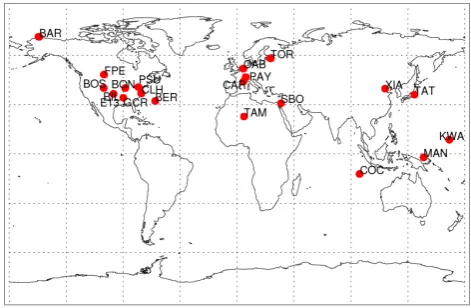
Fig. 4. BSRN stations used for the validation of the SCIAMACHY

surface solar irradiance (SSI) data in 2008 (except for the station SBO).

40 BSRN stations globally. However, not all the BSRN sta-tions have submitted the data measured in 2008 to the data archive; in total 20 stations were chosen for the validation. The BSRN stations used in the validation are shown in Fig. 4. More information about the BSRN stations can be found at the BSRN data center (http://www.bsrn.awi.de/). The BSRN stations at the Arctic and Antarctic were excluded, because there are no SCIAMACHY SSI data over snow/ice surface. The station SBO was not used for the validation, because the FRESCO effective cloud fraction is not accurate over bright surfaces in deserts due to the surface albedo problem (Fournier et al., 2006). Tamanrasset (TAM) is also located in the desert but the surface albedo at the Sahara desert has been corrected by Fournier et al. (2006); therefore this station has been included. Most of the selected stations are located in the Northern Hemisphere and cover a large range of surface types and topographic types.

The instantaneous SCIAMACHY SSI data were compared with the hourly mean BSRN global irradiances. According to Pinker et al. (2003), the best validation results can be ob-tained when both the satellite and ground-based observations are averaged over 1 h. Therefore, the measured 1-min BSRN global irradiances were averaged over 60 min centered on the SCIAMACHY overpass time to reduce large variance caused by broken cloud fields and to match the SCIAMACHY pixel size of 60×30 km2. From one year of data in 2008 we ob-tained 1006 collocated SCIAMACHY SSI and BSRN data points. The collocated data spanned from January to Decem-ber for most of the stations, but the data for BAR, PAY and XIA were only available from July to December, January to October and January to August, respectively.

882 P. Wang et al.: Surface solar irradiance from SCIAMACHY measurements: algorithm and validation

44 1

Figure 5. Instantaneous surface solar irradiances derived from SCIAMACHY (black line) 2

and the hourly mean BSRN global irradiances (red line) as a function of day of year for 3

every station. The number of cases is from January to December 2008, except for BAR, 4

PAY, XIA. 5

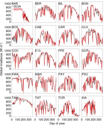
Fig. 5. Instantaneous surface solar irradiances derived from SCIAMACHY (black line) and the hourly mean BSRN global irradiances (red

line) as a function of day of year for every station. The cases are from January to December 2008, except for BAR, PAY, XIA.

solar zenith angle variation also improves the correlation. In general, the results are encouraging: good agreements are found between the SCIAMACHY SSI and BSRN data for all the stations. At tropical stations, e.g. COC, KWA, MAN, the global irradiances have small seasonal variations and the values are relatively large in all months. The ampli-tude of the seasonal variations for the global irradiances be-comes larger at higher latitudes with high values in summer and much lower values in winter. The SCIAMACHY SSI has a relative large negative bias at MAN, because the ef-fective cloud fraction is overestimated. The MAN station is located on an island with an area similar to the SCIA-MACHY pixel size but cannot be resolved in the GOME surface albedo database. Therefore, in FRESCO cloud re-trieval the surface albedo of ocean is used and the effective cloud fraction is overestimated. Although COC and KWA

45

1

Figure 6. Scatter plots of the instantaneous surface solar irradiances derived from

2

SCIAMACHY versus the hourly mean BSRN global irradiances for every station in

3

2008. Same data as in Fig. 5. The red lines indicate the one-to-one lines.

4

5

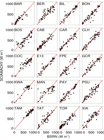
Fig. 6. Scatter plots of the instantaneous surface solar irradiances derived from SCIAMACHY versus the hourly mean BSRN global

irradi-ances for every station in 2008. Same data as in Fig. 5. The red lines indicate the one-to-one lines.

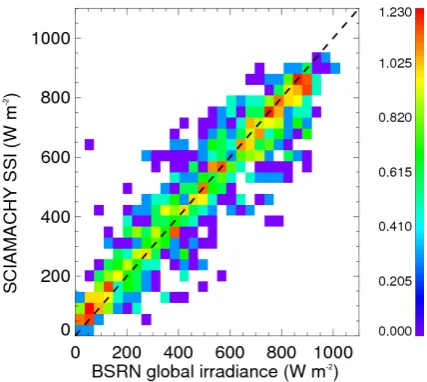
The scatter plots of SCIAMACHY SSI versus BSRN global irradiances are shown in Fig. 6 for every BSRN sta-tion. As illustrated in Fig. 6, most SCIAMACHY SSI and BSRN global irradiances are aligned along the one-to-one line. At TAM, the scatter is quite small, because there are hardly any clouds in the desert. The scatter density plot of all the validation data are shown in Fig. 7. There are a few outliers, but there is almost no bias. Because the clear-sky irradiances are calculated from the aerosol and water vapor monthly mean climatology data, the SSI variations caused by the water vapor and aerosol fluctuations on an hourly or daily scale cannot be revealed by the SCIAMACHY SSI

data. This could explain some differences between the in-stantaneous SCIAMACHY SSI and the hourly mean BSRN measurements. The scatter of the validation results is prob-ably mainly due to the large SCIAMACHY pixel size, par-ticularly at the pixels with a high frequency of broken clouds and at the coast.

884 P. Wang et al.: Surface solar irradiance from SCIAMACHY measurements: algorithm and validation

46 1

Figure 7. Scatter density plot of the instantaneous SCIAMACHY surface solar irradiance 2

(SSI) versus the hourly mean BSRN global irradiances for all the collocated data in 2008. 3

The dashed line is the one-to-one line. The color scale indicates the logarithm of the 4

number density of the data points. 5

6

7

8

9

10

11

12

13

Fig. 7. Scatter density plot of the instantaneous SCIAMACHY

sur-face solar irradiance (SSI) versus the hourly mean BSRN global irradiances for all the collocated data in 2008. The dashed line is the one-to-one line. The color scale indicates the logarithm of the number density of the data points.

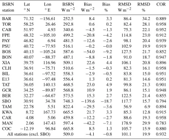
the mean of all stations. The averages of the hourly mean global irradiances generally increase from north to south be-sides the modulations due to clouds. The standard devia-tions for the hourly mean BSRN global irradiances are rel-atively large, often greater than 50 %, for nearly every sta-tion (not included in the table). This is a clear indicasta-tion of the large variations of clouds or broken clouds within the one hour time period. The bias and root mean square de-viation (RMSD) are quite different for every station, which agrees with the plots shown in Figs. 5 and 6. The RMSD between SCIAMACHY SSI and BSRN global irradiances are slightly correlated with the standard deviations of the BSRN hourly mean global irradiances (r= 0.35). The mea-surements at BIL and E13 were made at a few kilometers from each other and the bias, RMSD and correlation co-efficients were also similar for these two sites. This sug-gests the consistency of the BSRN and SCIAMACHY SSI data. The large negative bias of SCIAMACHY SSI at the SBO site suggests that the effective cloud fraction is too large and the surface albedo in the database could be too low. The SBO and TAM sites are both in desert regions. At SBO the mean effective cloud fraction of all the val-idation data is 0.314; however, at TAM the mean effec-tive cloud fraction is only 0.044. The SCIAMACHY SSI values at SBO are systematically lower than the BSRN measurements with a mean difference of −139.6 W m−2. The correlation coefficient between SCIAMACHY SSI and BSRN measurements is 0.794. This indicates that we have to improve the surface albedo database used in the FRESCO cloud retrieval algorithm. The mean global irradi-ance for all BSRN measurements is 509.0 W m−2. The mean

difference between SCIAMACHY SSI and BSRN global ir-radiances is −4.1 W m−2_{, which is −0.8 % of the mean} BSRN global irradiance. The RMSD of all the collocated data is 101.1 W m−2, corresponding to 19.9 % of the mean BSRN global irradiance. The correlation coefficient between the two data sets is 0.932 for 1006 data points.

4.2 Evaluation of monthly mean SCIAMACHY SSI with ISCCP-FD radiation data

In the previous section, SCIAMACHY SSI data have been validated with BSRN station data on an instantaneous ba-sis. The respective validation results have demonstrated the ability of the algorithm for the generation of SSI values with good accuracy. However, due to the relative low overpass frequency of SCIAMACHY, it is interesting to investigate how good SCIAMACHY SSI monthly means perform on a global scale in relation to existing and established climatolo-gies. Therefore, in this section SCIAMACHY SSI is com-pared with ISCCP-FD radiation data on a global scale.

Zhang et al. (2004) have produced an 18-year data set of radiative flux profiles (called ISCCP-FD) at 3-h time steps, global at 280-km intervals, that provides full- and clear-sky, shortwave and longwave, upwelling and downwelling fluxes at five levels (surface (SRF), 680 hPa, 440 hPa, 100 hPa, and TOA). The data set has been created by employing the NASA GISS climate Global Circulation Model (GCM) ra-diative transfer code and a collection of global data sets de-scribing the properties of the clouds and the surface at every 3 hours (using ISCCP products). The 280-km global inter-val can be converted into a 2.5◦_×2.5◦ _{regular latitude and} longitude grid. The comparisons of monthly, regional mean values from ISCCP-FD TOA and SRF fluxes with Earth Ra-diation Budget Experiment (ERBE), Clouds and the Earth’s Radiant Energy System (CERES) and BSRN values suggest that the overall uncertainties are 5–10 W m−2 at TOA and 10–15 W m−2at SRF (Zhang et al., 2004). The ISCCP-FD data set provides an independent global data set for the eval-uation of the SCIAMACHY SSI data set.

47

1

Figure 8. Zonal means of the SCIAMACHY surface solar irradiances (black) and the

2

ISCCP-FD surface shortwave downwelling fluxes (red) in January-December 2006. The

3

solid lines show the full-sky global irradiances (

G

) and the dotted lines illustrate the

4

clear-sky global irradiances (

G

).

5

6

7

8

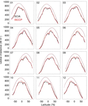
Fig. 8. Zonal means of the SCIAMACHY surface solar irradiances (black) and the ISCCP-FD surface shortwave downwelling fluxes (red)

in January–December 2006. The solid lines show the full-sky global irradiances (G) and the dotted lines illustrate the clear-sky global irradiances (G_clr).

the data sets for both situations. The clear-sky products were calculated without cloud input parameters, thus the clear- and full-sky products were identical at the grids without clouds.

The zonal means of the SCIAMACHY SSI and ISCCP-FD SDF are shown in Fig. 8 from January to December 2006. The clear-sky zonal mean global irradiances are also plotted for comparison. The SCIAMACHY SSI and ISCCP-FD SDF agree well with respect to large patterns although small dif-ferences appear at the tropical regions for both full-sky and clear-sky SSI. The SCIAMACHY SSI and ISCCP-FD SDF have good linear correlation for every month. The latitudi-nal variation of the solar zenith angle also contributes to the good linear correlation. The scatter density plots of SCIA-MACHY SSI and ISCCP-FD SDF for January and July are illustrated in Fig. 9 as examples. Most of the points are close

to the one-to-one line and the correlation coefficients are 0.97 and 0.98 for January and July, respectively. In July there are lots of low irradiance values at high latitude in the Southern Hemisphere, therefore in Fig. 9b the largest number density of the SSI values occurs close to 0 as one point. In July a large number of values are still along the one-to-one line. The RMSD values are 10.4 % and 9.6 % for January and July, respectively.

886 P. Wang et al.: Surface solar irradiance from SCIAMACHY measurements: algorithm and validation

48 1

Figure 9. Scatter density plots of the SCIAMACHY surface solar irradiances (SSI) versus 2

the ISCCP-FD surface shortwave downwelling fluxes (SDF) for (a) January and (b) July 3

2006. The dashed line is the one-to-one line. The color scale indicates the logarithm of 4

the number density of the data points. 5

6

7

Fig. 9. Scatter density plots of the SCIAMACHY surface solar irradiances (SSI) versus the ISCCP-FD surface shortwave downwelling fluxes

(SDF) for (a) January and (b) July 2006. The dashed line is the one-to-one line. The color scale indicates the logarithm of the number density of the data points.

1

2

Figure 10. Maps of the SCIAMACHY surface solar irradiances (SSI) and the ISCCP-FD

3

surface shortwave downwelling fluxes (SDF) for (a, b) January and (c, d) July 2006. The

4

white areas indicate the missing data due to snow/ice at the surface or solar zenith angles

5

larger than 89 degree.

6

7

8

9

10

11

12

13

14

Fig. 10. Maps of the SCIAMACHY surface solar irradiances (SSI) and the ISCCP-FD surface shortwave downwelling fluxes (SDF) for (a, b) January and (c, d) July 2006. The white areas indicate the missing data due to snow/ice at the surface or solar zenith angles larger than

89◦.

zonal means illustrated in Fig. 8. The SCIAMACHY SSI maps seem slightly noisier than the ISCCP-FD SDF maps, because of the relatively sparse global coverage of the SCIAMACHY measurements (namely global coverage in 6 days) while the ISCCP data have daily global coverage. The statistical results of the comparisons between SCIA-MACHY SSI and ISCCP-FD SDF are listed in Table 2. For the monthly mean clear-sky irradiances, SCIAMACHY SSI are slightly higher than ISCCP-FD SDF in the summer

months (June–September) with a maximum difference of +2 W m−2and lower than ISCCP-FD SDF for the rest of the year. Including clouds, SCIAMACHY SSI values are lower than ISCCP-FD SDF for all the months. The maximum of the differences is−11.67 W m−2(−2 %) and the maximum RMSD is 62 W m−2(12 %). However, the mean difference is still within the uncertainty of the ISCCP-FD SDF data. The correlation coefficients are larger than 0.96 for every month. The differences could be due to the input parameters, for

Table 1. Instantaneous SCIAMACHY SSI evaluation results using the BSRN global irradiances in 2008. Column 4: BSRN W m−2is the mean BSRN data used for validation at every station, the average of the BSRN data used in Figs. 5 and 6. Bias = SCIAMACHY SSI – BSRN, RMSD = root mean square deviation, COR = correlation.

BSRN Lat Lon BSRN Bias Bias RMSD RMSD COR station ◦N ◦E W m−2 W m−2 % W m−2 %

BAR 71.32 −156.61 252.5 8.4 3.3 86.4 34.2 0.889 TOR 58.25 26.46 292.8 0.6 0.2 82.4 28.1 0.958 CAB 51.97 4.93 340.6 −4.5 −1.3 75.3 22.1 0.952 FPE 48.32 −105.10 499.2 −20.8 −4.2 114.8 23.0 0.912 PAY 46.82 6.94 481.5 −12.6 −2.6 98.1 20.4 0.939 PSU 40.72 −77.93 516.1 −0.2 −0.0 102.9 19.9 0.919 BOS 40.13 −105.24 587.6 −54.0 −9.2 127.5 21.7 0.852 BON 40.07 −88.37 487.1 −8.8 −1.8 91.0 18.7 0.947 XIA 39.75 116.96 509.1 22.6 4.4 106.1 20.8 0.896 CLH 36.91 −75.71 510.6 −1.5 −0.3 82.3 16.1 0.958 BIL 36.61 −97.52 558.3 −2.9 −0.5 83.8 15.0 0.951 E13 36.61 −97.48 556.4 1.3 0.2 81.3 14.6 0.951 TAT 36.05 140.13 468.5 23.0 4.9 99.8 21.3 0.901 GCR 34.25 −89.87 568.8 10.9 1.9 86.1 15.1 0.948 BER 32.27 −64.67 573.5 15.3 2.7 122.5 21.4 0.855 SBO 30.91 34.78 748.3 −139.6 −18.7 117.7 15.7 0.794 TAM 22.78 5.51 822.4 −29.5 −3.6 56.9 6.9 0.894 KWA 8.72 167.73 665.5 21.7 3.3 85.3 12.8 0.915 CAR 4.08 5.06 459.8 −12.2 −2.7 88.6 19.3 0.958 MAN 2.06 147.43 597.4 −42.2 −7.1 178.9 29.9 0.783 COC −12.19 96.84 665.8 8.5 1.3 105.7 15.9 0.880 All stations (excl. SBO) 509.0 −4.1 −0.8 101.1 19.9 0.932

Table 2. Monthly mean SCIAMACHY SSI evaluation results using the ISCCP-FD surface shortwave downwelling fluxes for 2006.

Bias = SCIAMACHY SSI – ISCCP-FD, RMSD = root mean square deviation, COR = correlation, CLR = clear-sky.

Month ISCCP Bias Bias RMSD RMSD COR ISCCP Bias W m−2 W m−2 % W m−2 % CLR CLR W m−2 W m−2 1 517.9 −5.2 −1.0 53.6 10.4 0.969 713.6 −9.2 2 515.6 −5.2 −1.0 56.7 11.0 0.965 702.6 −9.9 3 523.4 −9.0 −1.7 55.4 10.6 0.971 694.7 −9.9 4 521.6 −7.0 −1.4 61.6 11.8 0.969 678.5 −7.1 5 509.4 −8.5 −1.7 57.9 11.4 0.974 658.7 −1.8 6 503.2 −7.6 −1.5 50.5 10.0 0.979 653.8 1.6 7 493.2 −10.1 −2.1 47.2 9.6 0.982 638.3 2.1 8 498.0 −4.5 −0.9 47.5 9.6 0.980 653.3 0.5 9 523.6 −3.7 −0.7 59.0 11.3 0.967 685.0 0.4 10 536.8 −11.7 −2.2 53.3 9.9 0.975 708.8 −0.9 11 547.9 −11.3 −2.1 60.0 11.0 0.968 735.1 −3.7 12 532.9 −9.5 −1.8 59.9 11.3 0.964 732.6 −7.1

example, cloud parameters, water vapor, aerosols and sur-face albedo, and the different algorithms. To understand all the differences between the SCIAMACHY SSI and ISCCP-FD SDF products, we would have to investigate the differ-ences between the algorithms and all the input data (Zhang

888 P. Wang et al.: Surface solar irradiance from SCIAMACHY measurements: algorithm and validation too high water vapor or aerosols values (from the

climatol-ogy databases) are used in the MAGIC algorithm.

4.3 Discussions

The geostationary satellite-based surface solar irradiances derived using different versions of the Heliosat algorithm have been extensively compared with the ground-based so-lar radiation measurements in Europe. The samen−k rela-tion is used in the Heliosat algorithm and FRESCO SSI al-gorithm, hence it can be expected that the FRESCO SSI per-forms well concerning its precision for instantaneous data. Indeed, the evaluated RMSD values of FRESCO SSI versus BSRN data are in the same order of magnitude as those found from the comparison of SSI derived from Meteosat using He-liosat or HeHe-liosat-like methods with ground-based measure-ments (e.g. Ineichen and Perez, 1999; Zelenka et al., 1999; Dagestad, 2004; Lorenz, 2007). This demonstrates the per-formance of the FRESCO SSI algorithm concerning its preci-sion. However, due to the low temporal resolution of SCIA-MACHY, outside of the polar regions we can not expect that the accuracy and uncertainty of the SCIAMACHY SSI prod-uct is similar to that of SSI daily and monthly means derived from geostationary satellites (Moeser and Raschke, 1984). In fact, a higher uncertainty and lower accuracy could be ex-pected in regions with a significant diurnal cycle of clouds, aerosols or water vapor.

In addition to the direct comparison with ISCCP-FD, a brief discussion of the SCIAMACHY SSI validation results in comparison with the NOAA/AVHRR products generated by the CM-SAF is given here. NOAA/AVHRR is a series of polar orbiting satellites with a significant higher spatial reso-lution than SCIAMACHY (4×4 km2 versus 60×30 km2). The CM-SAF radiation algorithm for the retrieval of the SSI from NOAA/AVHRR satellites also uses the MAGIC algorithm for the calculation of clear-sky irradiances, but the cloudy irradiances are calculated with a cloud model that requires detailed cloud parameters as input, which is completely different from the Heliosat method. Hollman et al. (2006) compared the CM-SAF AVHRR based sur-face shortwave global irradiances with several BSRN sta-tions within Europe. The mean bias error was larger than 10 W m−2 for more than 50 % of the investigated monthly means, a result of large bias values in the instantaneous data. These results indicate that the FRESCO SSI algorithm might be able to generate SSI products in a similar accuracy to that derived from NOAA/AVHRR, despite of the larger SCIA-MACHY pixel size. This is a remarkable result which has to be further investigated.

The accuracy of the SCIAMACHY SSI product could still be improved through the FRESCO cloud algorithm and MAGIC algorithm. Because SCIAMACHY can provide si-multaneously effective cloud fraction and water vapor at ev-ery pixel (No¨el et al., 2004; Schrijver et al., 2009), it would be possible to replace the water vapor climatology with the

retrieved water vapor per pixel. For the operational SCIA-MACHY SSI product, the effective cloud fraction will be re-trieved assuming the cloud albedo to be 0.95 instead of the conversion approach using Eq. (8). The effective cloud frac-tion will be improved by the use of a high resolufrac-tion surface albedo database, such as MERIS surface albedo database (Popp et al., 2011).

The FRESCO cloud retrieval algorithm is based on radia-tive transfer theory; therefore the FRESCO SSI algorithm can be applied to different satellite measurements as long as the effective cloud fraction can be derived. We already have 15 years of FRESCO effective cloud fraction time series pro-duced from GOME and SCIAMACHY measurements (Wang et al., 2010). Therefore, we can expect a consistent SSI time series constructed from different satellite measurements us-ing the FRESCO SSI algorithm as well. The FRESCO SSI algorithm could also use the effective cloud fractions re-trieved from other cloud algorithms, such as the O2-O2 al-gorithm (Acarreta et al., 2004) for OMI (Ozone Monitoring Instrument), and PMD algorithms for GOME, GOME-2 and SCIAMACHY with minor modifications. Such a time se-ries might be a good alternative or complement to global SSI data sets retrieved from NOAA/AVHRR. Due to the on-board solar calibration of GOME(-2), SCIAMACHY and OMI, a high potential for the construction of a climate data record with high stability and homogeneity is present.

5 Conclusions

The FRESCO SSI algorithm was developed to retrieve broadband surface solar irradiances using the Heliosat method. The cloud index required in the Heliosat method was replaced by the effective cloud fraction retrieved from the O2 A band measurements. In the FRESCO SSI algo-rithm, the FRESCO cloud algorithm retrieves effective cloud fraction, and then the MAGIC algorithm uses the output of the FRESCO cloud algorithm to calculate the broadband (0.2–4 µm) surface solar irradiance. The cloud albedo is as-sumed to be 0.95 in the FRESCO cloud algorithm, so that the effective cloud fraction value is close to the cloud index value and the Heliosatn−krelation can be used unchanged. Two years of surface solar irradiances from SCIAMACHY mea-surements were derived by utilizing the FRESCO SSI algo-rithm. This is the first time that the broadband surface solar irradiances are derived from SCIAMACHY measurements. The SSI product is also a new application of the effective cloud fraction.

−4.1 W m−2_{(−0.8 %) and the RMSD is 101 W m}−2_{(20 %)} for all the stations. The correlation coefficient is 0.93 for 1006 collocated data points. The monthly mean SCIA-MACHY SSI values were compared with the ISCCP-FD surface shortwave downwelling fluxes at a 2.5◦×2.5◦ grid for 2006. The monthly mean SSI from SCIAMACHY has a good agreement with the ISCCP-FD monthly mean data, with a correlation coefficient greater than 0.96 for every month. The largest difference in the global irradiances (SCIAMACHY-ISCCP) is about−12 W m−2(−2 %) and the RMSD is 62 W m−2(12 %).

The validation results indicate that the instantaneous SCIAMACHY SSI data might have similar accuracy as the CM-SAF NOAA/AVHRR SSI products. This might suggest that the lower spatial resolution is compensated by a more so-phisticated calibration or accurate cloud information. These hints have to be investigated and analyzed in more detail in a forthcoming paper. However, SCIAMACHY SSI has a small negative bias, mostly at tropical regions. The SCIA-MACHY SSI product over desert areas may not be reliable because of the coarse spatial resolution of the GOME sur-face albedo database. For areas above 4000 m the SCIA-MACHY SSI can be too low, because the surface height is not included in the algorithm. The SCIAMACHY SSI prod-uct could be improved by using the high resolution surface albedo derived from MERIS and by using simultaneous wa-ter vapor products from SCIAMACHY.

The FRESCO SSI algorithm is fast, robust and suitable for the operational processing of the SCIAMACHY data. With minor adjustments, the FRESCO SSI algorithm can be applied to GOME(-2), OMI and TROPOMI (Tropospheric Ozone Monitoring Instrument) in the future. Therefore, a consistent SSI time series can be constructed from the launch of GOME in 1995. We can also take advantage of the differ-ent overpass times of the satellites to derive the daily mean surface solar irradiances by the combination of the morning orbit (SCIAMACHY, GOME(-2)) and afternoon orbit (OMI, TROPOMI) measurements. The accuracy of the daily mean SSI would be better than the instantaneous product.

Acknowledgements. The authors would like to thank Ronald

van der A (KNMI) for processing the FRESCO cloud products, and Rob Roebeling and Erwin Wolters for discussions. The authors would like to thank all the BSRN station scientists: Ellsworth G. Dutton (BAR, BER, KWA), Charles Long (BIL, MAN, E13), John A. Augustine (BON, BOS, FPE, GCR, PSU), Wouter H. Knap (CAB), Jean-Philippe Morel (CAR), Fred M. Denn (CLH), Bruce Forgan (COC), Laurent Vuilleumier (PAY), Mohamed Mimouni (TAM), Nozomu Ohkawara (TAT), Ain Kallis (TOR), Xiangao Xia (XIA), Vera Lyubansky (SBO), Gert Koenig-Langlo (BSRN data archive) and the World Radiation Monitoring Center (WRMC) for providing the data. BSRN data were downloaded from http://www.bsrn.awi.de/en/data/. This work is supported by the ESA WACMOS (Water Cycle Multi-mission Observation Strategy) project.

Edited by: M. Weber

References

Acarreta, J. R., de Haan, J. F., and Stammes, P.: Cloud pressure retrieval using the O₂-O₂absorption band at 477 nm, J. Geophys. Res., 109, D05204, doi:10.1029/2003JD003915, 2004.

Bishop, J. K. and Rossow, W. B.: Spatial and temporal variability of global surface solar irradiance, J. Geophys. Res., 96, 1839–1858, 1991.

Bovensmann, H., Burrows, J. P., Buchwitz, M., Frerick, J., No¨el, S., Rozanov, V. V., Chance, K. V., and Goede, A. H. P.: SCIA-MACHY - Mission objectives and measurement modes, J. At-mos. Sci., 56(2), 127–150, 1999.

Cano, D., Monget, J., Albuisson, M., Guillard, H., Regas, N., and Wald, L.: A method for the determination of the global solar radiation from meteorological satellite data, Sol. Energy, 37, 31– 39, 1986.

Dagestad, K.-F.: Mean bias deviation of the Heliosat algorithm for varying cloud properties and sun-ground-satellite geometry, Theor. Appl. Climatol., 79, 215–224, doi:10.1007/s00704-004-0072-5, 2004.

Dagestad, K.-F.: Estimating global radiation at ground level from satellite images, PhD. thesis in meteorology at University of Bergen, Norway, May, 2005.

Dagestad, K.-F. and Olseth, J. A.: A modified algorithm for calcu-lating the cloud index, Sol. Energy, 81, 280–289, 2007. Darnell, W. L., Staylor, W. F., Gupta, S. K., and Denn, F. M.:

Esti-mation of surface insolation using sun-synchronous satellite data, J. Climate, 820–835, 1988.

Duerr, B. and Zelenka, A.: Deriving surface global irradiance over the Alpine region from METEOSAT Second Generation data by supplementing the HELIOSAT method, Int. J. Remote Sens., 30(22), 5821–5841, doi:10.1080/01431160902744829, 2009. Fournier, N., Stammes, P., de Graaf, M., van der A, R., Piters, A.,

Grzegorski, M., and Kokhanovsky, A.: Improving cloud infor-mation over deserts from SCIAMACHY Oxygen A-band mea-surements, Atmos. Chem. Phys., 6, 163–172, doi:10.5194/acp-6-163-2006, 2006.

Grzegorski, M., Wenig, M., Platt, U., Stammes, P., Fournier, N., and Wagner, T.: The Heidelberg iterative cloud retrieval utilities (HI-CRU) and its application to GOME data, Atmos. Chem. Phys., 6, 4461–4476, doi:10.5194/acp-6-4461-2006, 2006.

Hammer, A., Heinemann, D., Hoyer, C. R. K., Lorenz, E., Mueller, R., and Beyer, H.: Solar energy assessment using remote sensing technologies, Remote Sens. Environ., 86, 423–432, 2003. Hollmann, R., Mueller, R., and Gratzki, A.: CM-SAF surface

radi-ation budget: First results with AVHRR data, Adv. Space Res., 37, 2166–2171, 2006.

Ineichen, P. and Perez, R.: Derivation of cloud index from geosta-tionary satellites and application to the production of solar irradi-ance and daylight illuminirradi-ance data, Theor. Appl. Climatol., 64, 119–130, 1999.

890 P. Wang et al.: Surface solar irradiance from SCIAMACHY measurements: algorithm and validation

properties in aerosol component modules of global models, At-mos. Chem. Phys., 6, 1815–1834, doi:10.5194/acp-6-1815-2006, 2006.

Koelemeijer, R. B. A., Stammes, P., Hovenier, J. W., and de Haan, J. F.: A fast method for retrieval of cloud parameters using oxy-gen A band measurements from GOME, J. Geophys. Res., 106, 3475–3490, 2001.

Koelemeijer, R. B. A., de Haan, J. F., and Stammes, P.: A database of spectral surface reflectivity in the range 335–772 nm de-rived from 5.5 years of GOME observations, J. Geophys. Res., 108(D2), D24070, doi:10.1029/2002JD002429, 2003.

Kokhanovsky, A. A., Rozanov, V. V., Nauss, T., Reudenbach, C., Daniel, J. S., Miller, H. L., and Burrows, J. P.: The semianalytical cloud retrieval algorithm for SCIAMACHY I. The validation, At-mos. Chem. Phys., 6, 1905–1911, doi:10.5194/acp-6-1905-2006, 2006.

Lai, Y.-J., Chou, M.-D., and Lin, P.-H.: Parameterization of topo-graphic effect on surface solar radiation, J. Geophys. Res., 115, D01104, doi:10.1029/2009JD012305, 2010.

Li, Z., Leighton, H. G., Masuda, K., and Takashima, T.: Estimate of SW flux absorbed at the surface from TOA reflected flux, J. Climate, 317–330, 1993.

Lorenz, E.: Improved diffuse radiation model, MSG, Technical re-port of the project PVSAT-2 (D4.2b), Energy and semiconductor research laboratory, University of Oldenburg, 2007.

Loyola, D.: Automatic cloud analysis from polar-orbiting satellites using neural network and data fusion techniques, in: Proceedings of the IEEE international geoscience and remote sensing sympo-sium, IGARSS’2004, Anchorage, 4, 2530–2534, 2004. McArthur, L. J. B.: Baseline Surface Radiation Network (BSRN)

operations manual – Version 2.1, WMO/TD Rep. 879, World Clim. Res. Programme, World Meteorol. Org., Geneva, 2004. Meyer, R., Hoyer, C., Schillings, C., Trieb, F., Diedrich, E., and

Schroedter, M.: SOLEMI: a new satellite-based service for high-resolution and precision solar radiation data for Europe, Africa and Asia, in ISES Solar World Congress, 2003.

Moeser, W. and Raschke, E.: Incident solar radiation over Europe estimated from METEOSAT data, J. Clim. Appl. Meteorol., 23, 166–170, 1984.

Mueller, R., Dagestad, K., Ineichen, P., Schroedter-Homscheidt, M., Cros, S., Dumortier, D., Kuhlemann, R., Olseth, J., Pier-navieja, G., Resie, C., Wald, L., and Heinemann, D.: Rethinking satellite based solar irradiance modeling: the SOLIS clear-sky module, Remote Sens. Environ., 91, 160–174, 2004.

Mueller, R., Matsoukas, C., Gratzki, A., Hollmann, R., and Behr, H.: The CM-SAF operational scheme for the satellite based re-trieval of solar surface irradiance - a LUT based eigenvector hy-brid approach, Remote Sens. Environ., 113(5), 1012–1024, 2009. No¨el, S., Buchwitz, M., and Burrows, J. P.: First retrieval of global water vapour column amounts from SCIAMACHY mea-surements, Atmos. Chem. Phys., 4, 111–125, doi:10.5194/acp-4-111-2004, 2004.

Ohmura, A., Dutton, E. G., Forgan, B., Fr¨ohlich, C., Gilgen, H., Hegner, H., Heimo, A., K¨onig-Langlo, G., McArthur, B., M¨uller, G., Philipona, R., Pinker, R., Whitlock, C. H., Dehne, K., and Wild, M.: Baseline Surface Radiation Network (BSRN/WCRP): New precision radiometry for climate research, B. Am. Meteorol. Soc., 79, 2115–2136, 1998.

Perez, R., Seals, R., and Zelenka, A.: Comparing satellite remote sensing and ground network measurements for the production of site/time specific irradiance data, Sol. Energy, 60, 89–96, 1997. Perez, R., Aguiar, R., Collares-Pereira, M., Dumortier, D.,

Estrada-Cajigal, V., Gueymard, C., Ineichen, P., Littlefair, P., Lund, H., Michalsky, J., Olseth, J., Renne, D., Rymes, M., Skartveit, A., Vignola, F., and Zelenka, A.: Solar resource assess-ment: A review, in Solar Energy – The state of the art, num-ber ISBN 1 902916239, in: ISES Position Papers, pages, James & James Science Publishers, London, 497–562, 2001. Pinker, R. T. and Laszlo, I.: Modeling surface solar irradiance for

satellite applications on global scale, J. Appl. Meteorol., 31, 194– 211, 1992.

Pinker, R. T., Tarpley, J. D., Laszlo, I., Mitchell, K. E., Houser, P. R., Wood, E. F., Schaake, J. C., Robock, A., Lohmann, D., Cos-grove, B. A., Sheffield, J., Duan, Q., Luo, L., and Higgins, R. W.: Surface radiation budgets in support of the GEWEX Continental-Scale International Project (GCIP) and the GEWEX Americas Prediction Project (GAPP), including the North American Land Data Assimilation System (NLDAS) project, J. Geophys. Res., 108(D22), 8844, doi:10.1029/2002JD003301, 2003.

Popp, C., Wang, P., Brunner, D., Stammes, P., Zhou, Y., and Grzegorski, M.: MERIS albedo climatology for FRESCO+ O2 A-band cloud retrieval, Atmos. Meas. Tech., 4, 463–483,

doi:10.5194/amt-4-463-2011, 2011.

Rigollier, C., Levefre, M., and Wald, L.: The method Heliosat-2 for deriving shortwave solar radiation from satellite images, Sol. Energy, 77, 159–169, 2004.

Rothman, L. S., Jacquemart, D., Barbe, A., Benner, D. C., Birk, M., Brown, L. R., Carleer, M. R., Chackerian Jr., C., Chance, K., Coudert, L., Dana, V., Devi, V. M., Flaud, J. M., Gamache, R. R., Goldman, A., Hartmann, J. M., Jucks, K. W., Maki, A. G., Mandin, J. Y., Massie, S. T., Orphal, J., Perrin, A., Rins-land, C. P., Smith, M. A. H., Tennyson, J., Tolchenov, R. N., Toth, R. A., Vander Auwera, J., Varanasi, P., and Wagner, G.: The HITRAN 2004 molecular spectroscopic database, J. Quant. Spectrosc. Ra., 96, 139–204, 2005.

Schmetz, J.: Relationship between solar net radiative flux at the top of the atmosphere and at the surface, J. Atmos. Sci., 1122–1132, 1993.

Schrijver, H., Gloudemans, A. M. S., Frankenberg, C., and Aben, I.: Water vapour total columns from SCIAMACHY spectra in the 2.36 µm window, Atmos. Meas. Tech., 2, 561–571, doi:10.5194/amt-2-561-2009, 2009.

Stammes, P., Sneep, M., de Haan, J. F., Veefkind, J. P., Wang, P., and Levelt, P. F.: Effective cloud fractions from the Ozone Moni-toring Instrument: Theoretical framework and validation, J. Geo-phys. Res., 113, D16S38, doi:10.1029/2007JD008820, 2008. Su, Z., Dorigo, W., Fern´andez-Prieto, D., Van Helvoirt, M.,

Hunger-shoefer, K., de Jeu, R., Parinussa, R., Timmermans, J., Roebel-ing, R., Schr¨oder, M., Schulz, J., Van der Tol, C., Stammes, P., Wagner, W., Wang, L., Wang, P., and Wolters, E.: Earth observation Water Cycle Multi-Mission Observation Strategy (WACMOS), Hydrol. Earth Syst. Sci. Discuss., 7, 7899–7956, doi:10.5194/hessd-7-7899-2010, 2010.

Wang, P., Stammes, P., van der A, R., Pinardi, G., and van Roozen-dael, M.: FRESCO+: an improved O2 A-band cloud retrieval

algorithm for tropospheric trace gas retrievals, Atmos. Chem. Phys., 8, 6565–6576, doi:10.5194/acp-8-6565-2008, 2008. Wang, P., Fournier, N., van der A, R. and Stammes, P.: Fifteen

years of global cloud data derived from GOME and SCIA-MACHY oxygen A band measurements, Proceedings of ESA Living Planet Symposium, Bergen, Norway, 29 June–2 July, 2010.

Wang, P., Knap, W. H., and Stammes, P.: Cloudy sky shortwave ra-diative closure for a Baseline Surface Radiation Network site, J. Geophys. Res., 116, D08202, doi:10.1029/2010JD015141, 2011. Yang, K., Koike, T., Stackhouse, P., Mikovitz, C., and Cox, S. J.: An assessment of satellite surface radiation products for highlands with Tibet instrumental data, Geophys. Res. Lett., 33, L22403, doi:10.1029/2006GL027640, 2006.

Zelenka, A., Perez, R., Seals, R., and Reme, D.: Effective accu-racy of satellite-derived hourly irradiances, Theor. Appl. Clima-tol., 62, 199–207, 1999.

Zhang, Y.-C., Rossow, W. B., Lacis, A. A., Oinas, V., and Mishchenko, M. I.: Calculation of radiative fluxes from the surface to top of atmosphere based on ISCCP and other global data sets: Refinements of the radiative transfer model and the input data, J. Geophys. Res., 109, D19105, doi:10.1029/2003JD004457, 2004.

Zhang, Y., Rossow, W. B., and Stackhouse Jr., P. W.: Comparison of different global information sources used in surface radiative flux calculation: Radiative properties of the near-surface atmosphere, J. Geophys. Res., 111, D13106, doi:10.1029/2005JD006873, 2006.