RSI RANGE DETERMINATION USING CUBICAL DISTANCE CLASSIFICATION

44

OPTIMAL DG PLACEMENT FOR MAXIMUM LOSS

REDUCTION IN RADIAL DISTRIBUTION SYSTEM USING

ABC ALGORITHM

M.PADMA LALITHA1_{,N.SINARAMI REDDY}2_{V.C. VEERA REDDY}3

1_{IEEE Member,HOD, Department of Electrical & Electronics Engineering,Annamacharya Institute Of} Techonology & Sciences, Rajampet, A.P. Tel# +9848998643

2_{HOD, Department Of Mechanical Engineering,Annamacharya Institute Of Techonology & Sciences,} Rajampet, A.P. Tel# +9848998643

3_{Electrical & Electronics Engineering Dept , S.V.U.C.E,S.V.University,Tirupathi, A.P}

E-mail: [email protected], [email protected], [email protected]

ABSTRACT

Distributed Generation (DG) is a promising solution to many power system problems such as voltage regulation, power loss, etc. This paper presents a new methodology using a new population based meta heuristic approach namely Artificial Bee Colony algorithm(ABC) for the placement of Distributed Generators(DG) in the radial distribution systems to reduce the real power losses and to improve the voltage profile. A two-stage methodology is used for the optimal DG placement . In the first stage, single DG placement method is used to find the optimal DG locations and in the second stage, ABC algorithm is used to find the sizes of the DGs corresponding to maximum loss reduction. The proposed method is tested on standard IEEE 33-bus test system and the results are presented and compared with different approaches available in the literature. The proposed method has outperformed the other methods in terms of the quality of solution and computational efficiency.

Keywords : DG placement, Meta heuristic methods, ABC Algorithm, loss reduction, radial distribution system.

1. INTRODUCTION

Distributed generation is small-scale power generation that is usually connected to or embedded in the distribution system. The term DG also implies the use of any modular technology that is sited throughout a utility’s service to lower the cost of service [1]. The benefits of DG are numerous [2, 3] and the reasons for implementing DGs are rational use of energy, deregulation policy, diversification of energy sources, ease of finding sites for smaller generators, shorter construction times and lower capital costs of smaller plants and proximity of the generation plant to heavy loads. The reduction in gaseous emissions (mainly CO2) offered by DGs is major legal driver for DG implementation [4]. Numerous studies used different approaches to evaluate the benefits from DGs to a network in the form of loss reduction, loading level reduction [6-8].

45 algorithm and differential evolution. The other advantage is that the global search ability is implemented by introducing neighborhood source production mechanism which is similar to mutation process.

In this paper, locations of distributed generators are identified by single DG placement method[18] and ABC algorithm which takes the number and location of DGs as input has been developed to determine the optimal size(s) of DG to minimize real power losses in distribution systems. The advantages of relieving ABC method from determination of locations of DGs are improved convergence characteristics and less computation time. Voltage and thermal constraints are considered. The algorithm was tested on 33-Bus Distribution System [19].To demonstrate the effectiveness of proposed method, results are compared with different approaches available in the literature.

2. THEORETICAL BACKGROUND

The total I2R loss in distribution system having n number of branches is given by:

∑

=

=

n

i i

Lt

I

Ri

P

1

2 ₍₁₎

Here I

i is the magnitude of the branch current and R

i is resistance of the i th

branch respectively. The branch current has two components, active component (I

a) and reactive component (Ir). The loss associated with the active and reactive components of branch currents can be written as:

∑

=

=

n

i ai

La

I

Ri

P

1

2 ₍₂₎

∑

=

=

n

i ri

Lr

I

Ri

P

1

2 ₍₃₎

For a given configuration of a single-source radial network, the loss P

La cannot be minimized because all active power must be supplied by the source. However by placing DGs, this loss can be reduced. This paper presents a method to minimize this loss by placing DGs and thereby reduces the total loss in the distribution system.

3. IDENTIFICATION OF OPTIMAL DG

LOCATIONS BY SINGLE DG PLACEMENT ALGORITHM

This algorithm determines the optimal size and location of DG units that should be placed in the system to minimize loss. First optimum sizes of DG units for all nodes are determined for base case and best one is chosen based on the maximum loss saving. This process is repeated if multiple DG locations are required by modifying the base system by inserting a DG unit into the system one-by-one.

3.1. Methodology

Assume that a single-source radial distribution system with n branches and a DG is to be placed at bus m and α be a set of branches connected between the source and bus m. The DG produces active current IDG, and for a radial network it changes only the active component of current of branch set α. The currents of other branches are unaffected. Thus new active current Inew_ai of the ith _{branch is given by}

Inew_ai = Iai + DiIDG (4) where Di = 1; if branch i

∈

α

= 0; otherwise

The loss PLacom associated with the active component of branch currents in new system (when DG is connected) is given by

i DG i n i ai com

La

I

D

I

R

P

2 1

)

(

∑

=

+

=

(5)

The saving S is the difference between equation 3 and 5 and is given by

i c DG DG n

i i ai

com La La

R

I

D

I

I

D

P

P

S

)

2

(

2 1

+

−

=

−

=

∑

= (6)

The DG current IDG that provides maximum saving can be obtained from

∑

=

=

+

−

=

∂

∂

n

i i ai i DG i

DG

R

I

D

I

D

I

S

1

0

)

(

2

(7)

The DG current for maximum saving is

∑

∑

∑

∑

∈ ∈ = =

₌

₋

−

=

α α i i

i ai i

n

i i i n

i i ai i

DG

R

R

I

R

D

R

I

D

I

1

1 ₍₈₎

The corresponding DG size is

46 Vm is voltage magnitude of bus-m. The optimum size of DG at each bus is determined using eqn (9). Then saving for each DG is determined using eqn (6).The DG with highest saving is candidate location for single DG placement. When the candidate bus is identified and DG is placed, the process is repeated to identify subsequent buses for DG placement.

3.2. Algorithm for Single DG Placement

Step 1: Conduct load flow analysis for the

original system .

Step 2: Calculate IDG and DG size using

equations 8 & 9 for buses i=2…n.

Step 3: Determine saving using equation 6, for buses i=2…n.

Step 4: Identify the maximum saving and the corresponding DG size.

Step5: The corresponding bus is candidate bus where DG can be placed. Modify the active load at this bus and conduct the load flow again. Step 6: Check whether the saving obtain is more than 1kW. If yes, go to step 2. Otherwise, go to next step.

Step 7: print all the candidate locations to place DG sources and the sizes.

Since the DGs are added to the system one by one, the sizes obtained by single DG placement algorithm are local optima not global optimum solution. The global optimal solution is obtained if multiple DGs are simultaneously placed in the system by using ABC algorithm. This method is explained in next section.

4. IDENTIFICATION OF OPTIMAL DG

SIZES BY ABC ALGORITHM

4.1. ABC Algorithm

The colony of artificial bees contains three groups of bees: employed bees, onlookers and scouts. A bee waiting on the dance area for making decision to choose food source is called an onlooker and a bee going to the food source visited by it previously is named employed bee. A bee carrying out random search is called scout. In the ABC algorithm, first half of the colony consists of employed artificial bees and the second half constitutes the onlookers. For every food source, there is only one employed bee. The employed bee whose food source is exhausted by the employed and onlooker bees becomes a scout. At initialization stage, a set of food source positions are randomly selected by the bees and their nectar amounts are determined. These bees come into hive and share the nectar information of sources with the bees waiting on

the dance area within the hive. After sharing the information, every employed bee goes to the food source area visited by her at the previous cycle since that food source exists in her memory, and then chooses a new food source by means of visual information in the neighborhood of the present one. Then an onlooker prefers a food source area depending on the nectar information distributed by the employed bees on the dance area. As the nectar amount of a food source increases, the probability with which that food source is chosen by an onlooker increases, too. After arriving at the selected area, employed bee chooses a new food source in the neighborhood of the one in the memory depending on visual information. Visual information is based on the comparison of food source positions. When the nectar of a food source is abandoned by the bees, a new food source is randomly determined by a scout bee and replaced with the abandoned one. In this model, at each cycle one scout goes outside for searching a new food source and the number of

employed and onlooker bees were equal. The

probability Pi of selecting a food source i is determined by using

…..(10)

47 solution consists of d parameters and let Xi = (Xi1, Xi2, Xi3…… Xid) be a solution..In order to determine a solution vi in neighborhood of Xi, a solution parameter j and other solution Xk=(Xk1, Xk2, Xk3…… Xkd) are selected randomly. Except for the values of the selected parameter j, all other parameter values of vi are same as Xi ,i.e.,vi=( Xi1, Xi2 …… Xi(j-1), Xij, Xi(j+1), … Xid). The value vi of the selected parameter j in vi is determined by

….(11) where u is an uniform variate in [-1, 1]. If the resulting value falls outside the acceptable range of j, it is set to the corresponding extreme value in that range.

4.2. ABC Algorithm to find DG sizes

The proposed ABC algorithm for finding sizes of DGs at selected locations to minimize the real power loss is as follows:

1. Read the input data.

2. Construct initial Bee population Xij as each bee is formed by sizes of DG units

3. Evaluate fitness value for each employed bee by the formula

…..(12) 4. Initialize iteration=1.

5. Generate new population (solution) vij in the neighborhood of Xij for employed bees using equation (11) and evaluate them.

6. Apply selection process between Xiand vi.

7. Calculate the probability values Pi for the solutions Xiby means of their fitness values using

the equation (10).

8. Produce the new populations vifor the onlookers from the populations Xi, selected depending on Pi by applying roulette wheel selection process, and evaluate them.

9. Apply selection process for the onlookers between Xiand vi.

10. Determine the abandoned solution, if exists, and replace it with a new randomly produced solution Xifor the scout bees using the following equation

…(13)

11. Memorize the best solution achieved so far. If the difference between two successive values is less than specified value stop.

12. increase the iteration number by one. 13. if iterations are less than specified go to step 5, otherwise stop.

5. RESULTS AND DISCUSSION

First load flow is conducted for IEEE 33-bus test system. The power loss due to active component of current is 136.9836 kW and power loss due to reactive component of the current is 66.9252 kW. A program is written in “MATLAB” to implement single DG placement algorithm . For the first iteration the maximum saving is occurring at bus 6. The candidate location for DG is bus 6 with a loss saving of 92.1751 kW. The optimum size of DG at bus 6 is 2.4886 MW. By assuming 2.4886 MW DG is connected at bus 6 of base system and is considered as base case. Now the candidate location is bus 15with 0.4406 MW size and the loss saving is 11.4385 KW. This process is repeated till the loss saving is insignificant. The results are shown in Table I.

Table I:Single DG placement results iteration

No. Bus No. DG Size (MW) Saving (KW)

1 6 2.4886 92.1751

2 15 0.4406 11.4385

3 25 0.6473 7.6936

4 32 0.4345 8.1415

The candidate locations for DG placement are taken from single DG placement algorithm i.e. 6,15,25,32.With these locations, sizes of DGs corresponding to global solution are determined by using ABC Algorithm described in section 4. The sizes of DGs are dependent on the number of DG locations. Generally it is not possible to install many DGs in a given radial system. Here 4 cases are considered . In case I only one DG installation is assumed. In case II two DGs , in case III three DGS and in the last case four DGs are assumed to be installed. DG sizes in the four optimal locations, total real power losses before and after DG installation for four cases are given in Table II.

48

Table II:Results of IEEE 33 bus system

The last column in Table II represents the saving in Kw for 1 MW DG installation. The case with greater ratio is desirable. As the number of DGs installed is increasing the saving is also increasing. In case4 maximum saving is achieved but the number of DGs are four . Though case4 is optimal it is not economical by considering the

cost of installation of 4 DGs. But in view of reliability, quality and future expansion of the system it is the best solution.

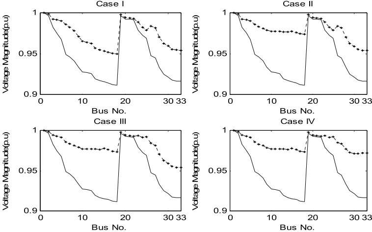
The voltage profile for all cases is shown in Figure 1. In all the cases voltage profile is improved and the improvement is significant.

Table III shows % improvements in power loss due to active component of branch current, reactive component of branch current and total active power loss of the system in the four cases considered. The loss due to active component of

branch current is reduced by more than 68% in least and nearly 96% at best. From Table III it is observed that the total real power loss is reduced by 48.5% in case 1 and 67% in case 4.

0 10 20 30 33

0.9 0.95 1

Bus No.

Vol

tag

e M

agni

tu

de(

p.

u)

Case I

0 10 20 30 33

0.9 0.95 1

Bus No.

Vol

tag

e M

agni

tu

de(

p.

u)

Case II

0 10 20 30 33

0.9 0.95 1

Bus No.

Vol

tage M

agn

itude(

p.

u)

Case III

0 10 20 30 33

0.9 0.95 1

Bus No.

Vol

tage M

agn

itude(

p.

u)

Case IV

Fig.1:Voltage profile with and without DG placement for all Cases Case bus _locations DG _sizes(Mw) Total _Size(MW)

losses before DG installation (Kw)

loss after DG

installation (Kw)

saving(Kw)

saving/ DG size

I 6 2.5775 2.5775

203.9088

105.0231 98.8857 39.9

II 6 1.9707 2.5464 89.9619 113.9469 44.75

15 0.5757

III

6 1.7569

3.1152 79.2526 124.6562 40.015

15 0.5757 25 0.7826

IV

6 1.0765

3.0884 66.5892 137.3196 44.86

49

Table III :Loss reduction by DG placement

case No.

P

La (kW) % Saving

P

Lr (kW) % Saving

P

Lt (kW) % Saving

Base case 136.98 ---- 66.9252 ---- 203.909 ----

Case1 43.159 68.49 61.8645 7.56 105.023 48.49

Case2 28.523 79.18 61.4392 8.2 89.9619 55.88

Case3 18.086 86.8 61.1657 8.6 79.2515 61.134

Case4 5.5676 95.94 61.0215 8.82 66.5892 67.34

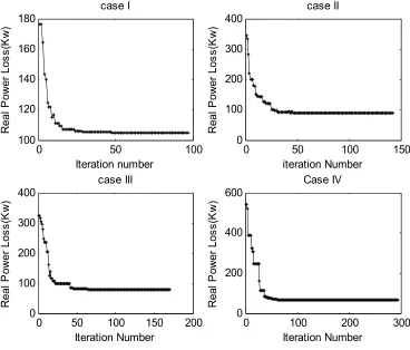
The convergence characteristics of ABC algorithm for all cases are shown in figure 2.

0 50 100

100 120 140 160 180

Iteration number

Re

al

P

owe

r

Lo

ss

(K

w

)

case I

0 50 100 150

0 100 200 300 400

iteration Number

Re

al

P

owe

r

Lo

ss

(K

w

)

case II

0 50 100 150 200

0 100 200 300 400

Iteration Number

R

eal

P

ow

er

Los

s(

K

w

)

case III

0 100 200 300

0 200 400 600

Iteration Number

R

eal

P

ow

er

Los

s(

K

w

)

Case IV

50 5.1. Comparison Performance

To demonstrate the validity of the proposed

method the results of proposed method is compared with an existing analytical method. The comparison is shown in Table IV.

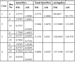
Table IV: Comparison between proposed method and other existing method.

Case Bus _No

sizes(Mw) Total Size(Mw) saving(Kw)

PM AM PM AM PM AM

1 6 2.5775

2.4886 2.5775 2.4886 98.8857 92.1751

2

6 1.9707 1.8981

2.5464 2.4676 113.9469 113.859 15 0.5757

0.5695

3

6 1.7569 1.6923

3.1152 3.034 124.6562 124.579 15 0.5757 0.5695

25 0.7826 _0.7722

4

6 1.0765 1.0188

3.0884 3.0107 137.3196 137.247 15 0.5757 0.5695

25 0.7824 0.7722

32 0.6538 0.6502

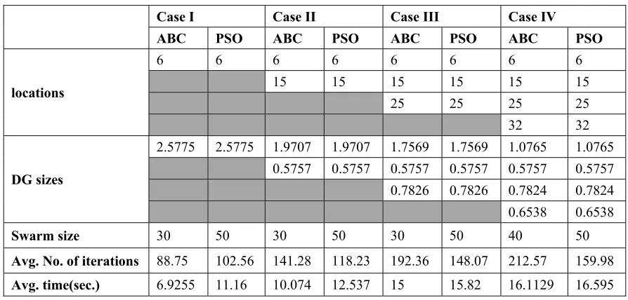
Savings by ABC algorithm are a little higher than the existing analytical method. The reason for this is in analytical method approximate loss formula is used. Table V shows comparison of voltage profile improvement by the two methods. The minimum voltage and % improvement in minimum voltage compared to base case for all the four cases, for the two methods discussed, are shown in the Table V. From the above tables it is clear that beyond producing the results that matches with those of existing method, proposed method has the added advantage of easy implementation of real time constraints on the system like time varying loads, different types of DG units etc., to effectively apply it to real time operation of a system. To demonstrate the supremacy of the proposed method the results are compared with the results of PSO algorithm as shown in Table VI. Both methods gives same sizes for DGs for all cases.Though the number of iterations are more

for ABC algorithm it takes less computation time because of its simplicity when compared to PSO method .

Table V: Comparison of Voltage improvement

case No. Min Voltage % improvement PM AM PM AM Base

case 0.9118 ---

case1 0.9498 0.9486 2.149 1.985

case2 0.9543 0.9596 2.533 2.358

case3 0.9544 0.9621 2.533 2.358

51

Table VI: Comparison of results of ABC and PSO algorithms

Case I Case II Case III Case IV

ABC PSO ABC PSO ABC PSO ABC PSO

locations

6 6 6 6 6 6 6 6 15 15 15 15 15 15

25 25 25 25

32 32

DG sizes

2.5775 2.5775 1.9707 1.9707 1.7569 1.7569 1.0765 1.0765 0.5757 0.5757 0.5757 0.5757 0.5757 0.5757

0.7826 0.7826 0.7824 0.7824

0.6538 0.6538

Swarm size 30 50 30 50 30 50 40 50

Avg. No. of iterations 88.75 102.56 141.28 118.23 192.36 148.07 212.57 159.98

Avg. time(sec.) 6.9255 11.16 10.074 12.537 15 15.82 16.1129 16.595

6. CONCLUSIONS

In this paper, a two-stage methodology of finding the optimal locations and sizes of DGs for maximum loss reduction of radial distribution systems is presented. Single DG placement method is proposed to find the optimal DG locations and ABC algorithm is proposed to find the optimal DG sizes.

The validity of the proposed method is proved from the comparison of the results of the proposed method with other existing methods. The results proved that the ABC algorithm is simple in nature than GA and PSO so it takes less computation time. By installing DGs at all the potential locations, the total power loss of the system has been reduced drastically and the voltage profile of the system is also improved. Inclusion of the real time constrains such as time varying loads and different types of DG units and discrete DG unit sizes into the proposed algorithm is the future scope of this work.

REFERENCES

[1]. G. Celli and F. Pilo, “Optimal distributed generation allocation in MV distribution networks”, Power Industry Computer Applications, 2001. Pica 2001. Innovative Computing For Power - Electric Energy Meets The Market. 22nd IEEE Power Engineering Society International Conference,May 2001,pp.81-86.

[2]. P. Chiradeja, R. Ramakumar, “An approach to quantify the technical benefits of distributed generation” IEEE Trans Energy Conversion,vol.19, no.4,pp.764-773,2004.

[3]. R.E. Brown, J. Pan, X. Feng, and K. Koutlev, “Siting distributed generation to defer T&D expansion,” Proc. IEE. Gen, Trans and Dist,vol.12, pp.1151-1159,1997.

[4]. E. Diaz-Dorado, J. Cidras, E. Miguez, “Application of evolutionary algorithms for the planning of urban distribution networks of medium voltage”, IEEE Trans. Power Systems , vol.17,no.3, pp.879-884,Aug 2002.

[5]. M. Mardaneh, G. B. Gharehpetian, “Siting and sizing of DG units using GA and OPF based technique,” TENCON. IEEE Region

10 Conference

,vol.3,pp.331-334,21-24,Nov.2004.

[6]. Silvestri A.Berizzi, S.Buonanno,

“Distributed generation planning using genetic algorithms” Electric Power

Engineering, Power Tech Budapest 99,

Inter. Conference, pp.257,1999.

52 [8]. G.Celli,E.Ghaini,S.Mocci and F.Pilo, “A

multi objective evolutionary algorithm for the sizing and sitting of distributed generation”, IEEE Transactions on power systems, vol.20,no.2,pp.750-757,May 2005.

[9]. G.Carpinelli,G.Celli, S.Mocci and F.Pilo,”Optimization of embedded sizing and sitting by using a double trade-off method”, IEE proceeding on generation, transmission and distribution,vol.152,no.4, pp.503-513, 2005.

[10]. C.L.T.Borges and D.M.Falcao, “Optimal distributed generation allocation for reliability,losses and voltage improvement”, International journal of power and energy systems,vol.28.no.6,pp.413-420,July 2006.

[11]. Wichit Krueasuk and Weerakorn Ongsakul, “Optimal Placement of Distributed Generation Using Particle Swarm Optimization”,M.Tech Thesis,AIT,Thailand.

[12]. B. Basturk, D. Karaboga, “An artificial bee colony (ABC) algorithm for numeric function optimization,” IEEE Swarm

Intelligence Symposium 2006, May12–

14,Indianapolis,IN,USA, 2006.

[13]. D. Karaboga, B. Basturk, “A powerful and efficient algorithm for numerical function optimization: artificial bee colony (ABC)

algorithm”, Journal of Global

Optimization,Vol. 39, pp.459–471,2007.

[14]. D. Karaboga, B. Basturk, “On the performance of artificial bee colony algorithm”, Applied Soft Computing Vol.8,pp.687–697,2008.

[15]. M.Padma Lalitha,V.C.Veera Reddy, N.Usha “Optimal DG placement for maximum loss reduction in radial distribution system” International journal of emerging technologies and applications in engineering, technology and sciences,Vol.2,issue-2,July-Dec

2009,pp.719-723.